Context: Like part 1, this comes out of Andrej Karpathy’s Becoming a Backprop Ninja (Part 4 of the spelled-out intro series), where you hand-write every backward pass instead of calling
.backward(). These notes are the longer explanation I want on hand the next time I go back to the video. If you have not watched it, start there:

This is a follow-up to Why the Gradient of a Broadcast Subtraction Is a Sum. Same setup, same style, different operator. Last time the forward pass copied a value, and the backward pass had to sum. This time the forward pass selects a value, and the backward pass has to do the opposite of selecting.
A 2x2 matrix is enough to see everything, so let us use one.
The forward pass
A = | A11  A12 |
    | A21  A22 |
Take the max of each row. Two rows go in, two numbers come out, so the result B is a 2x1 column:
B1 = max(A11, A12)
B2 = max(A21, A22)
To make this concrete, assume A11 > A12 in the first row, and A22 > A21 in the second. I deliberately picked different winning columns so the pattern that emerges is not a coincidence of symmetry. So:
B1 = A11
B2 = A22
Notice what happened to A12 and A21. They were read, they were compared, and then they were discarded. Their values do not appear anywhere in B.
The key insight
Upstream gives us G = dL/dB, shape 2x1, with elements G1 and G2. We need dL/dA, which must be 2x2.
Here is the whole thing in one observation: locally, B1 is not some blend of A11 and A12. It literally is A11.
Nudge A11 up by a tiny epsilon and B1 goes up by exactly epsilon, because A11 is still the larger of the two and still wins.
Nudge A12 up by a tiny epsilon and B1 does not move at all. A12 was losing before and it is still losing. The output does not know anything happened.
So the local derivatives are as simple as they get:
dB1/dA11 = 1 dB1/dA12 = 0
There is no partial credit here. max is a step function in disguise: within a small neighborhood of the current values, it is just a wire connected to the winner.
Applying the chain rule to both rows:
dL/dA11 = G1 * 1 = G1        dL/dA12 = G1 * 0 = 0
dL/dA21 = G2 * 0 = 0         dL/dA22 = G2 * 1 = G2
The computational graph
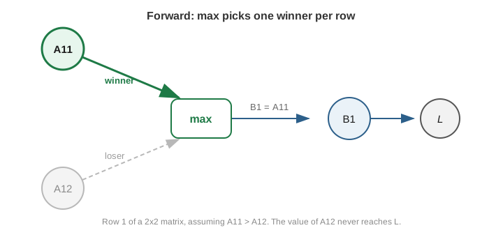
Take just the first row. Forward, both A11 and A12 are inputs to the max node, but only one of them survives it:
Now reverse the arrows. The gradient G1 comes back from L, passes through B1, reaches the max node, and then takes only one of the two available exits:
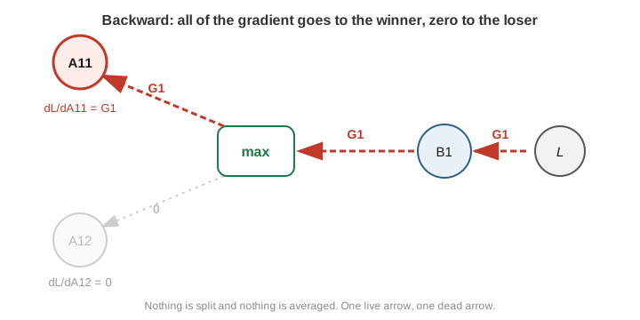
One live arrow and one dead arrow. Compare that to part 1, where B1 had two live arrows arriving and they had to be added together. Different forward structure, different backward structure, same chain rule producing both.
Writing it as a matrix
Doing this element by element is fine for a 2x2 but hopeless in real code. The vectorized form uses a one-hot mask: a matrix the same shape as A, with a 1 at each row’s argmax and 0 everywhere else.
M = | 1  0 |        row 1 argmax is column 0
    | 0  1 |        row 2 argmax is column 1
Then broadcast G back across the columns and gate it with the mask. That is elementwise multiplication:
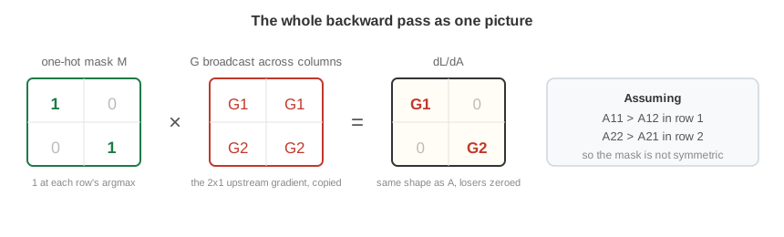
The broadcast in the middle is exactly the copy operation from part 1, showing up again from the other direction. Here it is doing the work of getting a 2x1 gradient back out to a 2x2 shape.
In PyTorch, the mask is literally what one_hot gives you:
import torch
import torch.nn.functional as F

idx = A.argmax(dim=1)                                  # which column won, per row
M = F.one_hot(idx, num_classes=A.shape[1]).float()     # the mask
dA = M * G                                             # G is (2, 1), broadcasts across columns
That is the entire backward pass for a row-wise max in three lines.
Two things worth knowing
Ties. If two elements in a row are exactly equal, max is not differentiable there. There is a corner in the function and no single slope. Frameworks resolve this by picking one index, usually the first, and giving it all the gradient. That is a legitimate subgradient choice, not a bug, and in practice exact ties in floating point are rare enough that it never comes up.
Losers really do get nothing. A12 gets a gradient of exactly zero through this path. No small nudge, no encouragement to try harder next time. If that path is the only route from A12 to the loss, it receives no update at all this step. This is the same mechanism behind dead ReLUs, where a unit stuck on the flat side of max(0, x) stops learning entirely. Gating operations route gradients, and anything not on the selected route gets nothing.
Verifying it
import torch
import torch.nn.functional as F

A = torch.randn(2, 2, requires_grad=True)
B = A.max(dim=1, keepdim=True).values     # shape (2, 1)

G = torch.randn(2, 1)
B.backward(G)

M = F.one_hot(A.argmax(dim=1), num_classes=2).float()
print(torch.allclose(A.grad, M * G))      # True
The pair of rules
Two posts, two operators, and the pattern behind both is about counting paths:
- Forward copies (broadcast), so backward sums. One input reached the loss by several routes, and the chain rule adds over routes.
- Forward selects (max), so backward scatters into the winner and zeroes the rest. The losers reached the loss by no route at all.
The shape argument works for both, too. Part 1 had to squeeze a 3x3 gradient down into 3x1, so it summed. Here we have to expand a 2x1 gradient back out to 2x2, so we broadcast and then mask. Before doing any calculus, look at the two shapes and ask which direction you are going. That alone tells you which operation to reach for.
And these two rules are not academic. The standard numerically stable softmax starts with:
logits - logits.max(dim=1, keepdim=True).values
which is a row-wise max feeding a broadcast subtraction. Backpropagating that single line requires both of these rules, one after the other.