How linear attention works: a small memory matrix and the gated delta rule

What if attention could read the past from a small matrix instead of revisiting an ever-growing list of keys and values?

Linear attention keeps a fixed-size memory matrix. The incoming token’s query reads from it; the token’s key and value update it. The gated delta rule adds a way to fade old information and correct particular associations. We can follow the whole calculation with a small example: two key features, three value features, and just six numbers in memory.

Contents

• From ordinary attention to a small memory
• What every dimension means
• Reading the memory with a query
• Writing a key-value association
• The gated delta rule
• One complete update with numbers
• A runnable check
• Why it is called linear attention
• References

From ordinary attention to a small memory

In ordinary causal attention, the current token has a query. We compare it with the keys of tokens up to and including the current position, turn those scores into softmax weights, and mix their value vectors. Each weight is one number multiplying an entire value vector.

For token t, that looks like:

score for token j = dot(k_j, q_t) / sqrt(d_k)
weights = softmax(scores for j <= t)
output = sum over j <= t of weight_j * v_j

The KV cache saves those keys and values. A new query still reads the permitted history.

To see the basic linear-attention idea, start with a simpler weighting rule: use the key-query dot product directly, without softmax. Leave out the constant score scale for this walkthrough. Then:

y_t = sum over j <= t of v_j * (k_jᵀ q_t)
    = sum over j <= t of (v_j k_jᵀ) q_t
    = S_t q_t

S_t = sum over j <= t of v_j k_jᵀ

The middle step is just associativity. The same query multiplies every term, so we can add the outer-product matrices first and multiply by the query once. That accumulated matrix is S, the memory.

This changes the attention rule; it is not an exact rearrangement of softmax attention. Softmax’s exponentials and query-dependent denominator prevent this simple factoring. FlashAttention preserves softmax and improves its execution; linear attention changes what is computed.

The classic linear-attention paper uses feature maps of queries and keys and keeps an additional running vector for normalization. Here we follow the simpler, unnormalized matrix-memory formulation used to introduce Gated DeltaNet in Section 2.1 of its paper. The gated delta rule below does not add a softmax denominator.

What every dimension means

We are looking at one head in one layer, for one sequence. Each such head and sequence has its own state. All vectors below are columns.

Q and K have the same head dimension, because their components must line up for a dot product. The value dimension need not match it. In a sequence-wide value matrix V, with tokens stored as rows, the shape would be T × d_v, where T is the number of tokens. Vdim is its feature width, not its token count.

S has one row per value feature and one column per key feature. These are feature axes, not lists of cached tokens. S combines information from many tokens into the same six entries.

The model obtains q, k, and v from learned transformations of the current token’s hidden representation. The output y is a contextualized head output, not a token ID or the complete model-width representation. Later processing combines heads and projects their outputs back into the model.

Reading the memory with a query

Suppose the current memory and query are:

      key features
         1   2
S = [    3   0    ]   value feature 1
    [    1   2    ]   value feature 2
    [    2   1    ]   value feature 3

q = [0.6]
    [0.8]

Multiplying S by q takes a dot product with each row:

y₁ = 3 * 0.6 + 0 * 0.8 = 1.8
y₂ = 1 * 0.6 + 2 * 0.8 = 2.2
y₃ = 2 * 0.6 + 1 * 0.8 = 2.0

Those subscripts name output components, not different tokens. Together they form one output vector, [1.8, 2.2, 2.0]ᵀ.

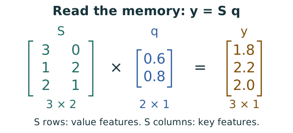
For basic additive linear attention, expanding S shows what the query is reading: a sum of earlier values, each weighted by its key’s dot product with q. We no longer need to visit every earlier token separately. With GDN, we read the same kind of matrix, but its contents have also been decayed and edited.

Writing a key-value association

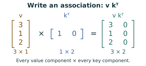
To write to S, multiply the value column by the transposed key row, v kᵀ. The superscript ᵀ means transpose: it turns a column into a row. This is an outer product, not a dot product:

(Vdim × 1) times (1 × headdim)
        = Vdim × headdim
        = 3 × 2

For v = [3, 1, 2]ᵀ and k = [1, 0]ᵀ:

v kᵀ = [3] [1  0] = [3  0]
       [1]           [1  0]
       [2]           [2  0]

Every value component multiplies every key component. A second pair, k = [0, 1]ᵀ and v = [0, 2, 1]ᵀ, writes the second column. Adding the two outer products gives the S we just read.

Basic linear attention therefore has a simple recurrence, starting from zero:

S_t = S_(t-1) + v_t k_tᵀ
y_t = S_t q_t

Update first, then read. That includes the current token, as causal self-attention normally does. The previous state is carried forward across tokens and processing batches within the same sequence.

But what if another token uses the same key with a new value? Simple addition mixes old and new. If a note says “the robot moved,” we would prefer to update its remembered location rather than add the two locations together. The gated delta rule provides that targeted update.

The gated delta rule

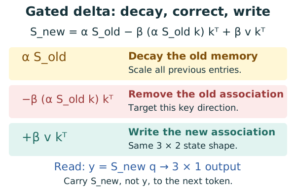
GDN means Gated DeltaNet. Its update combines decay with a targeted correction. With value features as rows and key features as columns, Equation 10 is:

Here α (alpha) is a scalar decay gate, β (beta) is a scalar writing strength, and I is the d_k × d_k identity matrix, 2 × 2 here. The model computes the gates from the current input. In the paper, their values lie between zero and one; endpoints below are useful limiting cases. The paper also L2-normalizes queries and keys, making their lengths one.

Decay the old memory

First form a decayed memory:

D = α_t S_(t-1)

Alpha near one retains most of the old memory. Alpha near zero clears most of it. It scales all the old entries, not just the current key’s direction. The new write on the right of the equation is not multiplied by alpha.

Correct the association at this key

Read the decayed memory using the key, not the query:

prediction = D k_t
error = v_t - prediction

This asks, “What value does the memory currently associate with this key?” The error tells us how far that answer is from the incoming value. Write the error back along the key:

S_t = D + β_t (v_t - D k_t) k_tᵀ

Expanding that expression gives D (I - β_t k_t k_tᵀ) + β_t v_t k_tᵀ, the same gated delta rule. The subtraction removes part of the old association; the addition supplies the replacement.

For a unit-length key, kᵀk = 1, so reading the updated memory at that same key gives:

S_t k_t = (1 - β_t) D k_t + β_t v_t

Beta one replaces the association completely. Beta one-half moves it halfway toward the new value. Beta zero leaves only the decay.

“Same key” means a direction in feature space, not a dictionary lookup. The targeted edit leaves an orthogonal key direction alone, but overlapping directions can be affected. Alpha’s earlier global decay still applies to both.

Write the new value along the key

The final term, β_t v_t k_tᵀ, writes a key-value association, not another column or a new entry in a growing token list. Its shape is still 3 × 2.

Finally, use the incoming token’s query to read the updated state:

y_t = S_t q_t

The distinction is useful: k chooses where to edit; q chooses what to read. Their dimensions match, but their values need not.

One complete update with numbers

Reuse our state. The incoming token has k = [1, 0]ᵀ and a new value v = [0, 4, 1]ᵀ. Choose α = 0.5 and β = 1: fade the memory, then fully replace this key’s association.

S_old = [3  0]       D = 0.5 S_old = [1.5  0  ]
        [1  2]                     [0.5  1  ]
        [2  1]                     [1    0.5]

prediction = D k = [1.5, 0.5, 1]ᵀ
error = v - prediction = [-1.5, 3.5, 0]ᵀ

β error kᵀ = [-1.5  0]
             [ 3.5  0]
             [ 0    0]

S_new = D + β error kᵀ = [0  0  ]
                        [4  1  ]
                        [1  0.5]

We can also check I - β k kᵀ directly. Here k kᵀ = [[1, 0], [0, 0]], so I - k kᵀ = [[0, 0], [0, 1]]. Right-multiplying D by that matrix wipes its first column and preserves its second. Adding v kᵀ fills the first column with the new value.

Reading with [1, 0]ᵀ now returns [0, 4, 1]ᵀ, the replacement. Reading with the orthogonal [0, 1]ᵀ returns [0, 1, 0.5]ᵀ: the other association survived the targeted edit, but was halved by alpha.

For our mixed query q = [0.6, 0.8]ᵀ, the final output is:

y = S_new q = [0, 3.2, 1.0]ᵀ

That is the contextualized Vdim × 1 output for this head.

A runnable check

This NumPy example checks both forms of the GDN equation. @ means matrix multiplication; np.outer makes the column-times-row product.

import numpy as np

S = np.array([[3., 0.], [1., 2.], [2., 1.]])
q = np.array([0.6, 0.8])
k = np.array([1., 0.])
v = np.array([0., 4., 1.])
alpha, beta = 0.5, 1.0

# Factored gated delta equation.
direct = S @ (alpha * (np.eye(2) - beta * np.outer(k, k)))
direct += beta * np.outer(v, k)

# The same update as decay, predict, and correct.
decayed = alpha * S
prediction = decayed @ k
updated = decayed + beta * np.outer(v - prediction, k)
y = updated @ q

assert np.allclose(direct, updated)
assert np.allclose(updated @ k, v)
assert np.allclose(y, [0., 3.2, 1.])
print(updated)
print(y)

Output:

[[0.  0. ]
 [4.  1. ]
 [1.  0.5]]
[0.  3.2 1. ]

NumPy uses one-dimensional arrays for the vectors here; the operations implement the column-vector convention above. The example isolates the recurrence, not the surrounding learned projections, normalization, and output gating of a complete GDN layer.

Why it is called linear attention

With head dimensions fixed, each token updates and reads a d_v × d_k matrix. The recurrent mixing work is O(d_v d_k) per token, or O(T d_v d_k) over T tokens. Its persistent matrix state has no token axis, so it does not grow with the sequence length. This describes the recurrent path, not every buffer used during training or every layer of a hybrid model.

The factored GDN formula contains a square matrix, but the error-update form avoids constructing it or doing a full matrix-matrix multiply: use a matrix-vector read and a rank-one outer-product write. Implementations can also process chunks to exploit GPU parallelism.

The tradeoff is that a fixed-size state cannot retain arbitrarily many independent associations perfectly. Similar keys can interfere. GDN makes that memory more useful by learning when to fade old information and when to correct a particular association.

The core idea is simple: read the memory with q, and update it with k and v. The gates decide how much to retain and how strongly to replace an association.

References

• Angelos Katharopoulos and colleagues, Transformers are RNNs: Fast Autoregressive Transformers with Linear Attention (2020). Associative computation, kernel feature maps, normalization, and recurrent evaluation. Paper · PDF.
• Songlin Yang, Jan Kautz, and Ali Hatamizadeh, Gated Delta Networks: Improving Mamba2 with Delta Rule (ICLR 2025). Section 2.1 gives the matrix-memory convention; Equation 10 gives the gated delta rule; Sections 3.3 and 3.4 discuss chunkwise computation and the model block. Paper, v3 · PDF, v3 · Official code.