What does llama.cpp's KV cache actually look like in memory?

I wanted to see what llama.cpp’s KV cache actually looks like in memory, so I dumped the cached keys and values for a short prompt in Qwen3-0.6B, a small model with 28 layers. I used an RTX 4090, an F16 cache, and a context capacity of 4,096 tokens.

The useful picture is fairly simple: every layer has its own K and V tensors, every occupied row holds one token’s numbers, and streams add another dimension. Here is that picture, followed down to an actual pair of bytes in the dump.

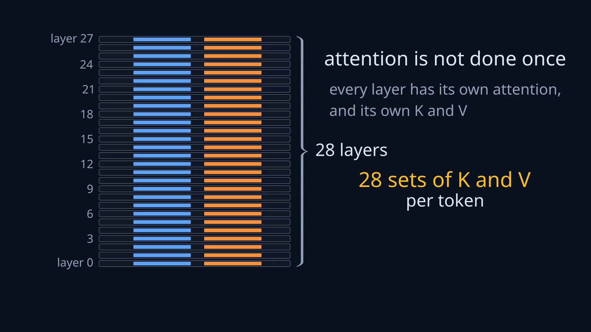
28 layers, 56 tensors

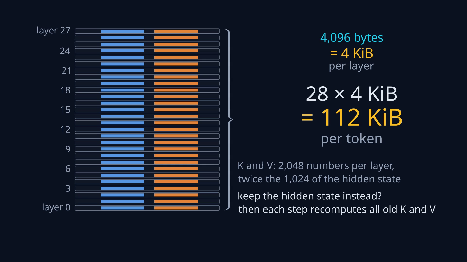
Attention happens in every one of this model’s 28 layers. Each layer computes its own keys and values, so the cache keeps 28 K tensors and 28 V tensors: 56 tensors in all.

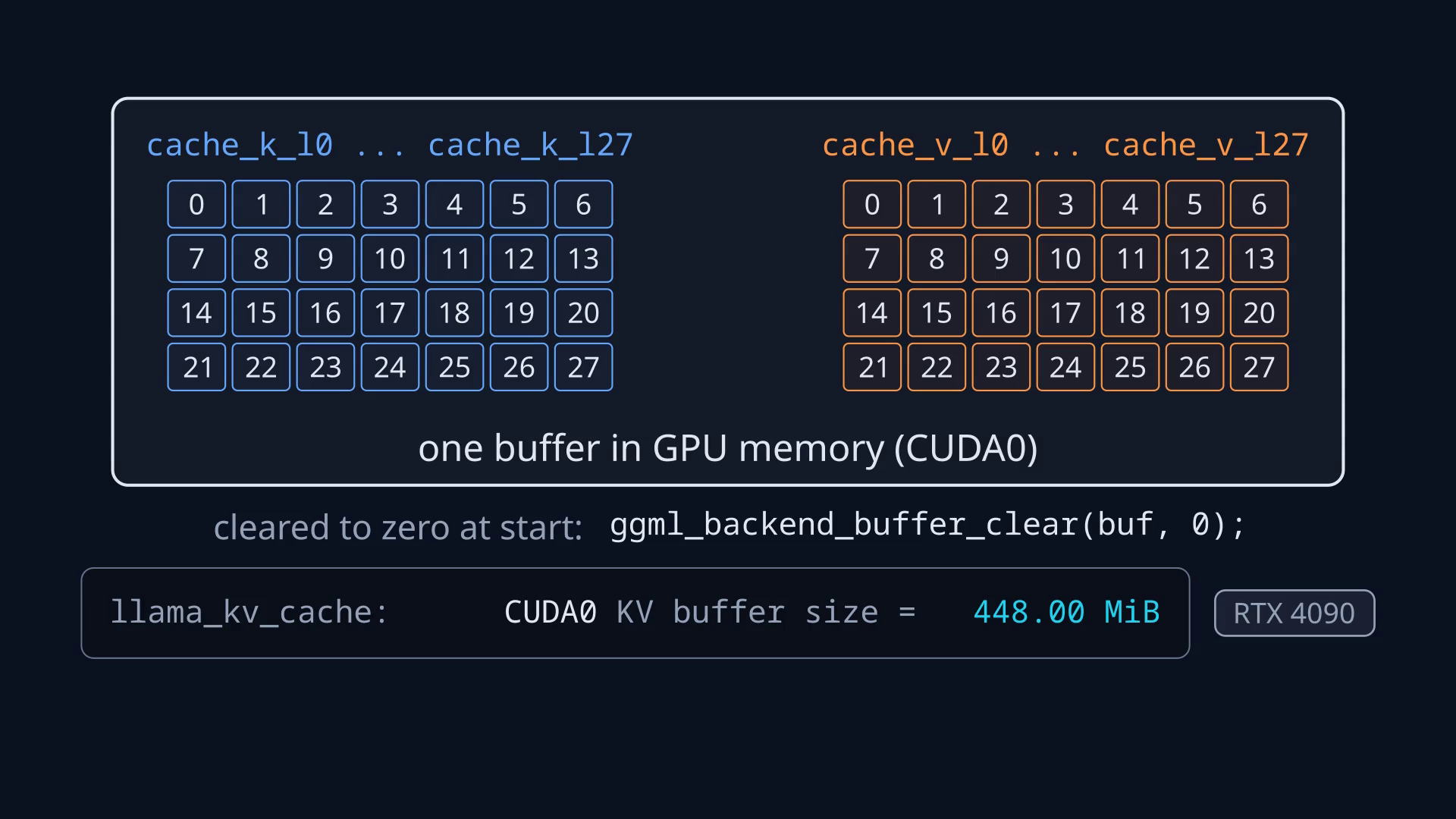
A stack of 28 model layers, each with its own blue K and orange V storage. — Each token contributes keys and values at every layer. Blue is K, orange is V. Click any diagram to see it at full size.

With all layers offloaded to the GPU, these tensors live in one CUDA buffer. The diagram groups the keys and values by color; it is an inventory, not their address order. In this build, the live buffer contains the layer pairs in order: K0, V0, K1, V1, .... The saved file uses a different order, which we will see below.

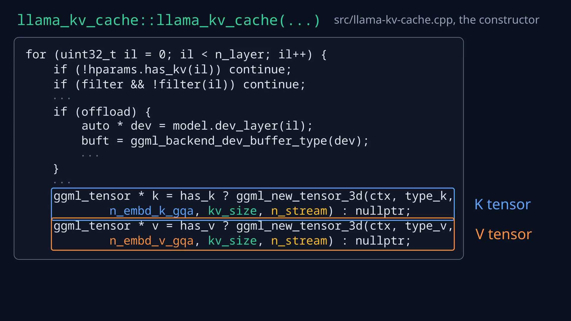
All 28 K tensors and 28 V tensors grouped inside one 448 MiB CUDA0 allocation. — The 56 tensors share one GPU buffer in this all-GPU run.

The constructor creates the two tensors inside its layer loop. For this model, the relevant calls are:

ggml_new_tensor_3d(ctx, type_k,
                   n_embd_k_gqa, kv_size, n_stream);
ggml_new_tensor_3d(ctx, type_v,
                   n_embd_v_gqa, kv_size, n_stream);

The constructor and per-layer structure

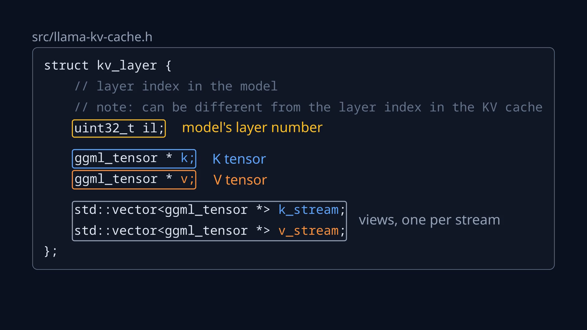
The llama_kv_cache constructor loops over layers and creates one three-dimensional K tensor and one V tensor for each included layer. — The layer loop and the two tensor allocations.

The kv_layer structure holds the model layer index, K and V tensor pointers, and per-stream views. — `kv_layer` keeps the pair of tensors and their stream views together.

One row, one token’s keys

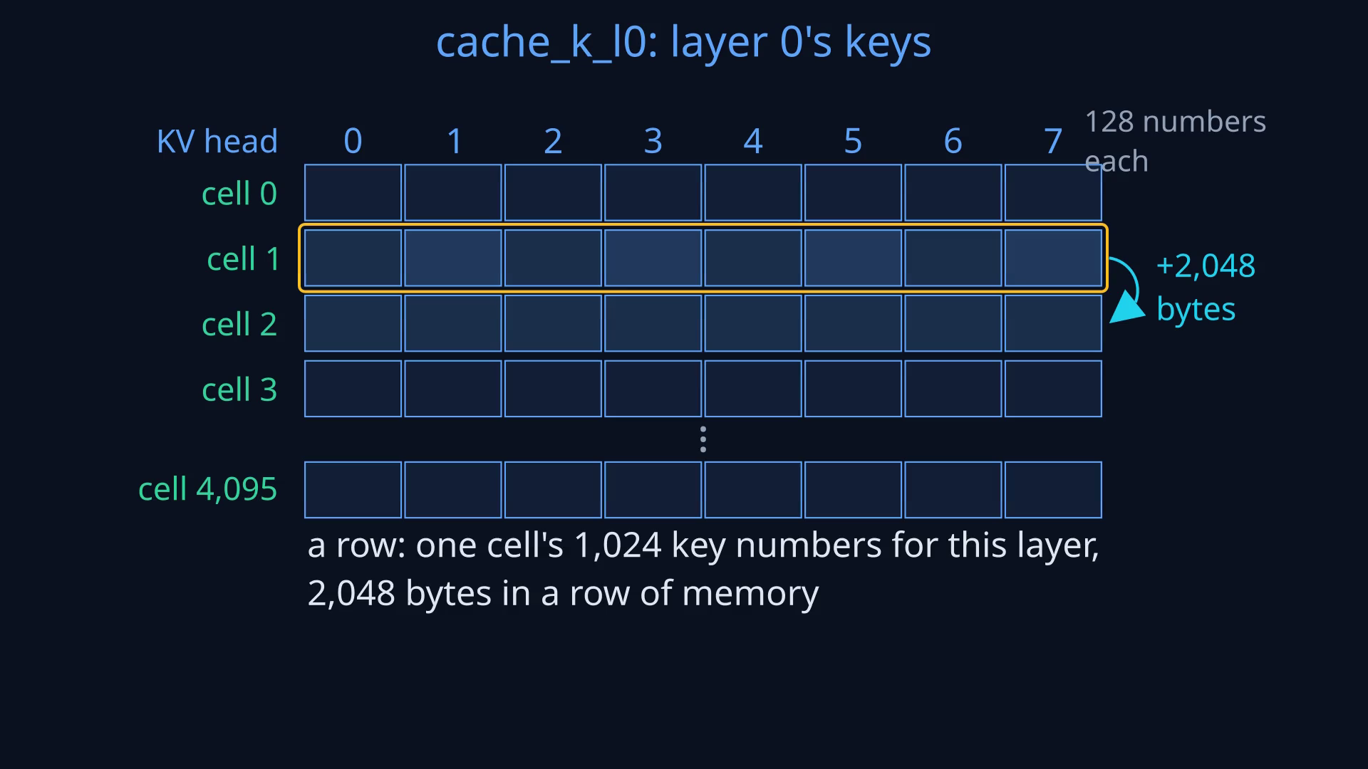
For one token in one layer, K contains 1,024 numbers. That is eight KV heads with 128 numbers each, packed next to each other in a row. V has the same size. Each F16 number takes two bytes, so a K row occupies 2,048 bytes, or 2 KiB. A V row takes another 2 KiB.

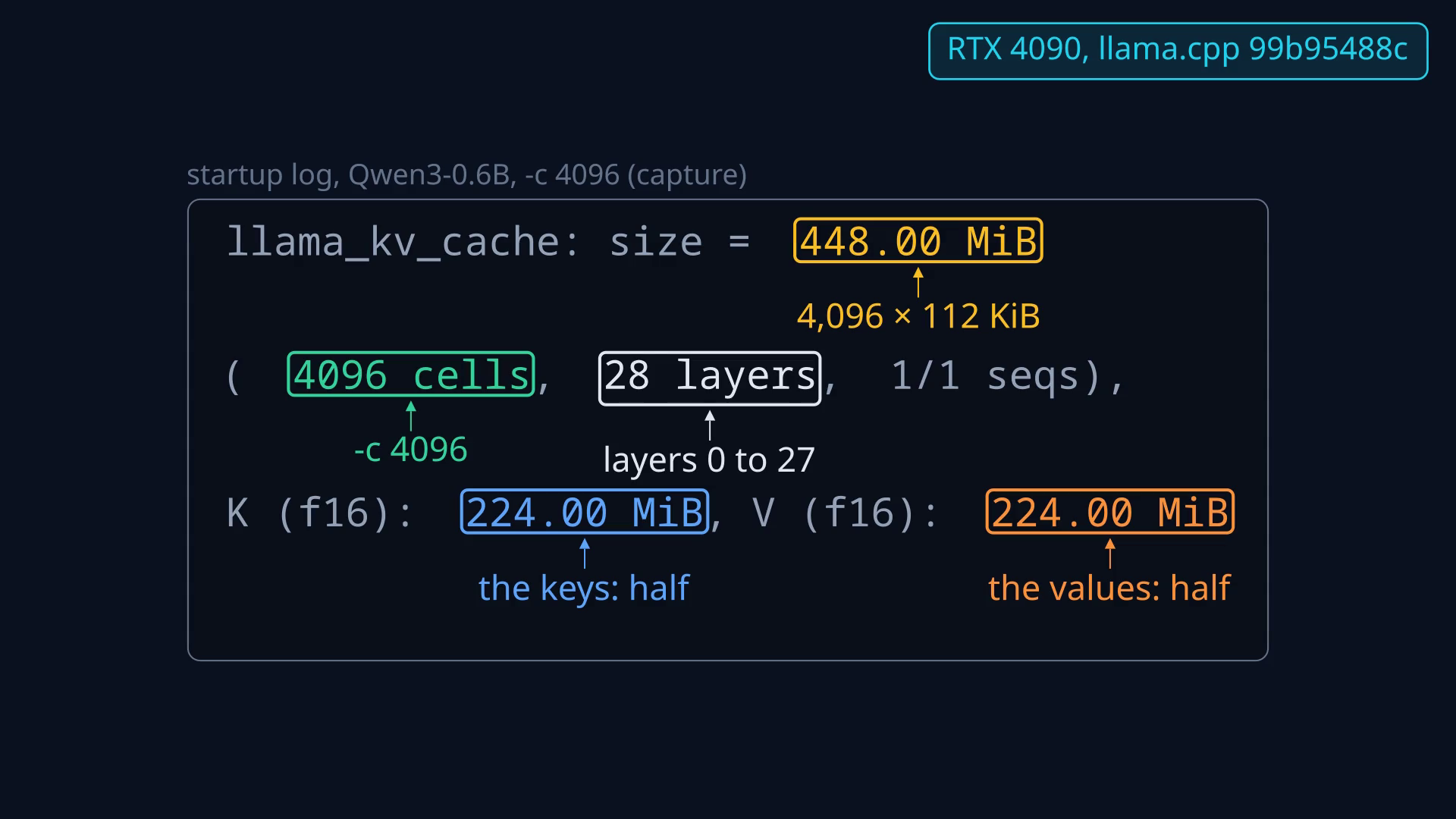
Rows of the layer-zero K tensor. Each row contains eight KV heads of 128 values, and the next row begins 2048 bytes later. — One row holds a token's keys for this layer. The eight heads sit side by side.

The dimensions in the model's startup log

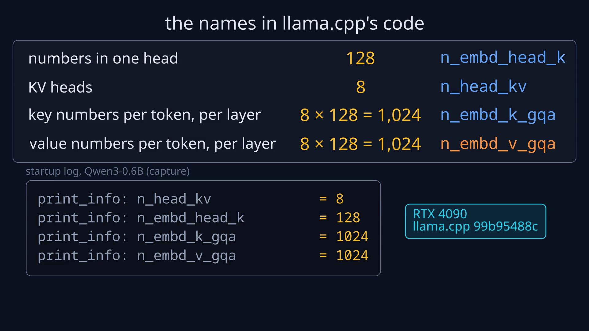
Startup output: eight KV heads, head size 128, and 1024 K and V values per token per layer. — `n_embd_k_gqa = n_head_kv × n_embd_head_k = 8 × 128 = 1024`.

Across all 28 layers, one token’s K and V payload is:

2 KiB × 28 layers × 2 (K and V) = 112 KiB

For c cache cells, the total is c × 112 KiB. So even eight tokens hold 896 KiB, almost a MiB, in this small model. Here KiB means 1,024 bytes and MiB means 1,024 KiB.

Two 2 KiB rows make 4 KiB per layer; 28 layers make 112 KiB of cached keys and values per token. — 4 KiB per layer, multiplied by 28 layers.

llama.cpp reserves space for the configured capacity, rather than growing this buffer one token at a time. My -c 4096 run therefore reserved 448 MiB, even though the prompt only occupied seven cells.

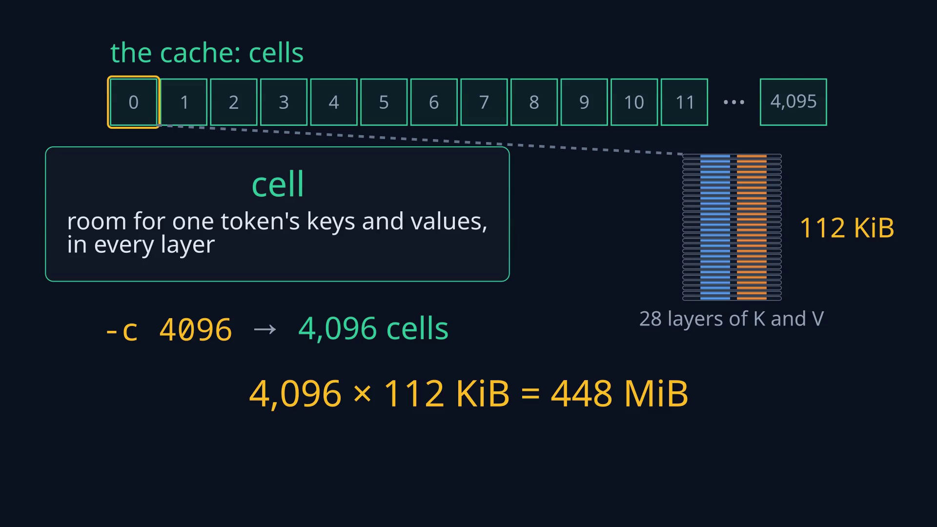
4096 cache cells, each representing room for a token's K and V across all 28 layers, total 448 MiB. — A cell is a shared row index across the layers' tensors, not one contiguous 112 KiB chunk.

The measured allocation

The real startup log reports 448 MiB: 224 MiB for F16 keys and 224 MiB for F16 values, over 4096 cells and 28 layers. — The startup log agrees with the calculation: 224 MiB of K plus 224 MiB of V.

Opening the .bin dump

For the experiment, I fed in “The cat sat on the mat.”, which became seven tokens, and saved sequence 0’s occupied cache across all 28 layers. I used a small helper, kvprobe, with the following command:

./kvprobe -m Qwen3-0.6B-Q8_0.gguf \
  -c 4096 -ngl 99 -fa on -ctk f16 -ctv f16 \
  --ops 'text:0:The cat sat on the mat.;save:0:state-f16.bin'

python3 parse_state.py state-f16.bin --cells 3

The model’s weights are Q8_0; the cache in this experiment is F16. The helper saves the state through llama.cpp’s API:

const size_t n = llama_state_seq_get_size_ext(
    ctx, s, LLAMA_STATE_SEQ_FLAGS_NONE);
std::vector<uint8_t> buf(n);
const size_t got = llama_state_seq_get_data_ext(
    ctx, buf.data(), buf.size(), s,
    LLAMA_STATE_SEQ_FLAGS_NONE);
std::ofstream(path, std::ios::binary).write(
    (const char *) buf.data(), (std::streamsize) got);

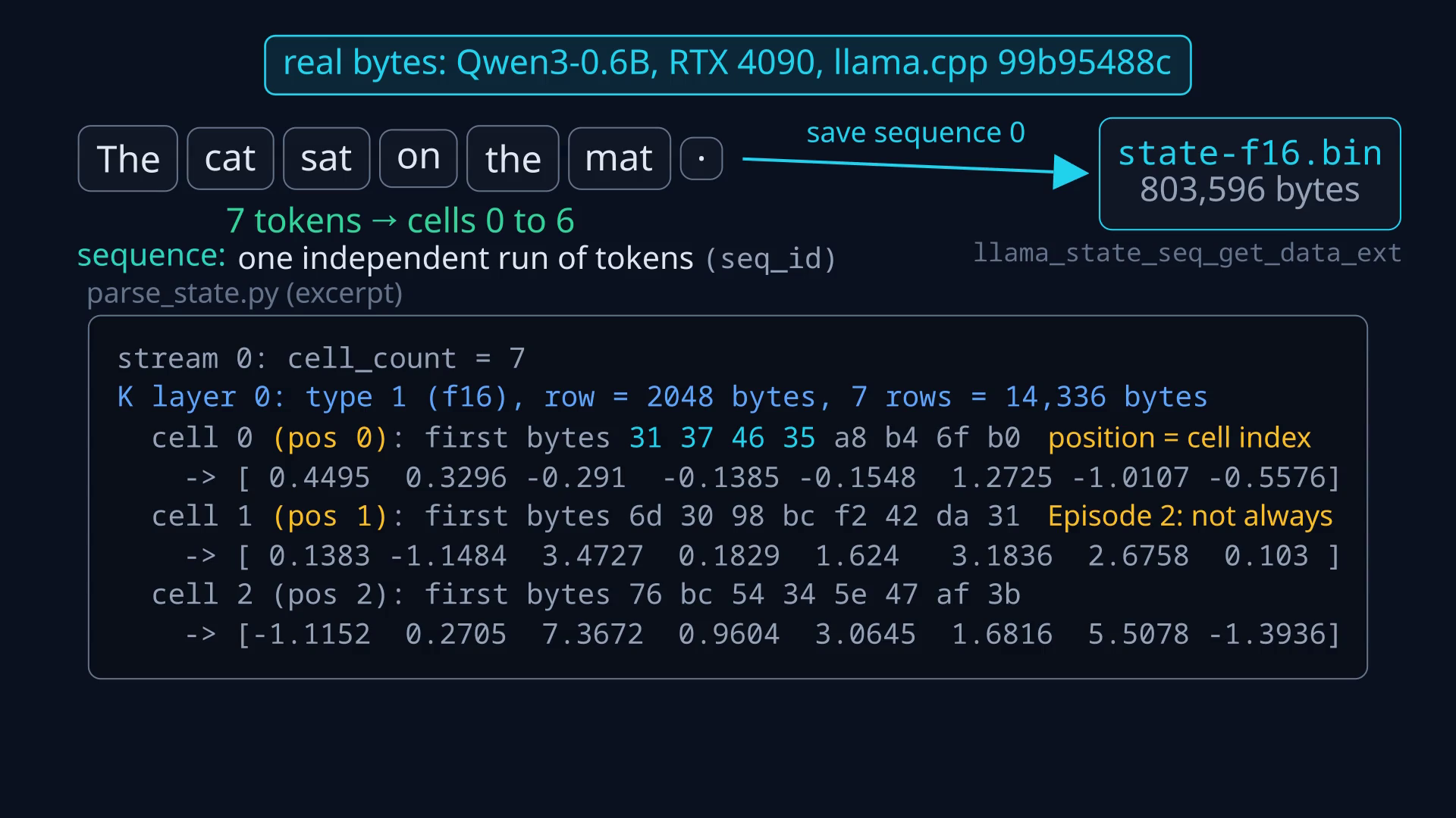
The seven-token sentence is saved to state-f16.bin; the parser displays actual K rows and their hexadecimal bytes. — The saved sequence contains seven occupied rows per tensor, not all 4,096 reserved rows.

In the saved file, the K records run from layer 0 through layer 27, followed by the V records for all 28 layers. Each record has a small header and then its seven rows. This is where the “all K, then all V” layout appears.

metadata
K0, K1, ... K27   (header + 7 rows in each record)
V0, V1, ... V27   (header + 7 rows in each record)

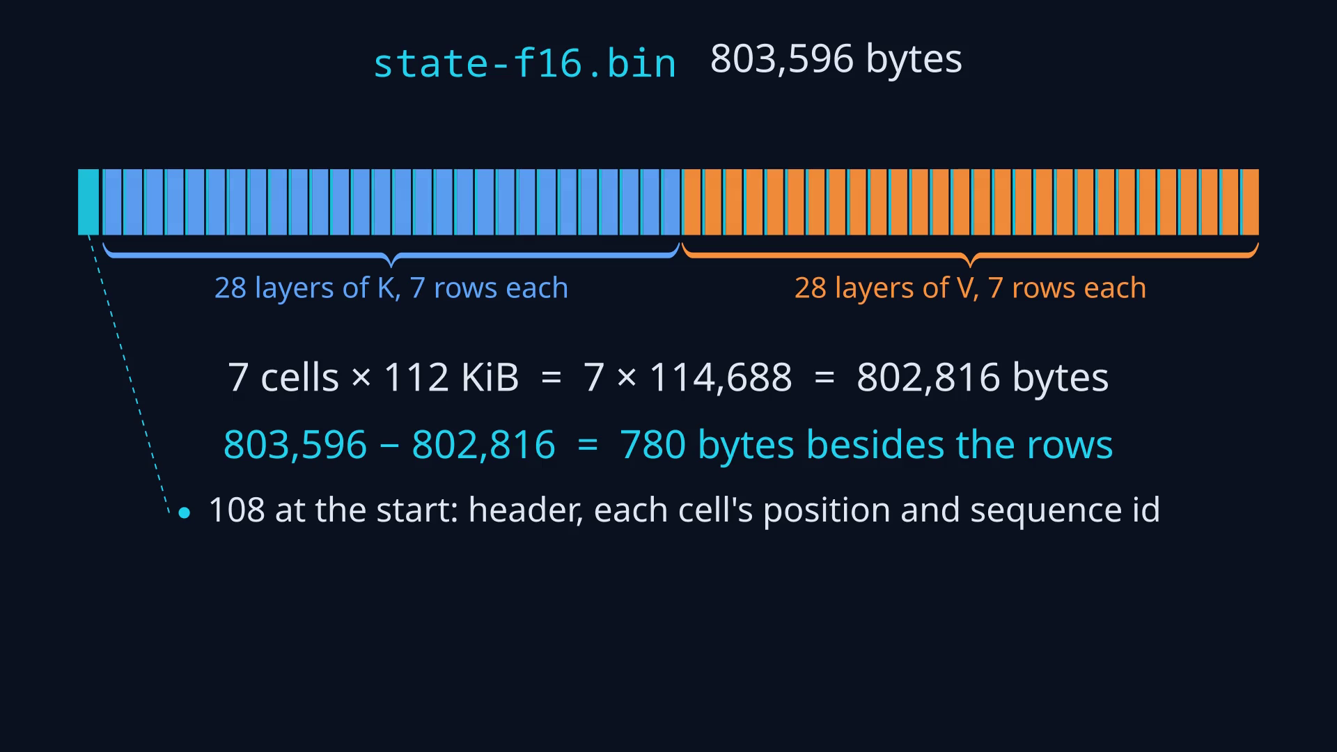
The serialized file contains 28 blue K records followed by 28 orange V records. Seven cells contribute 802816 payload bytes; metadata brings the file to 803596 bytes. — The file contains 802,816 bytes of K/V data and 780 bytes of metadata, for a total of **803,596 bytes**.

The first K record starts at byte 108. Its 12-byte header puts the first actual K value at byte 120. Reading four F16 numbers directly from there gives:

import struct
from pathlib import Path

data = Path("state-f16.bin").read_bytes()
print(len(data))
print(data[120:128].hex(" "))
print(tuple(round(x, 4) for x in
            struct.unpack_from("<4e", data, 120)))

803596
31 37 46 35 a8 b4 6f b0
(0.4495, 0.3296, -0.291, -0.1385)

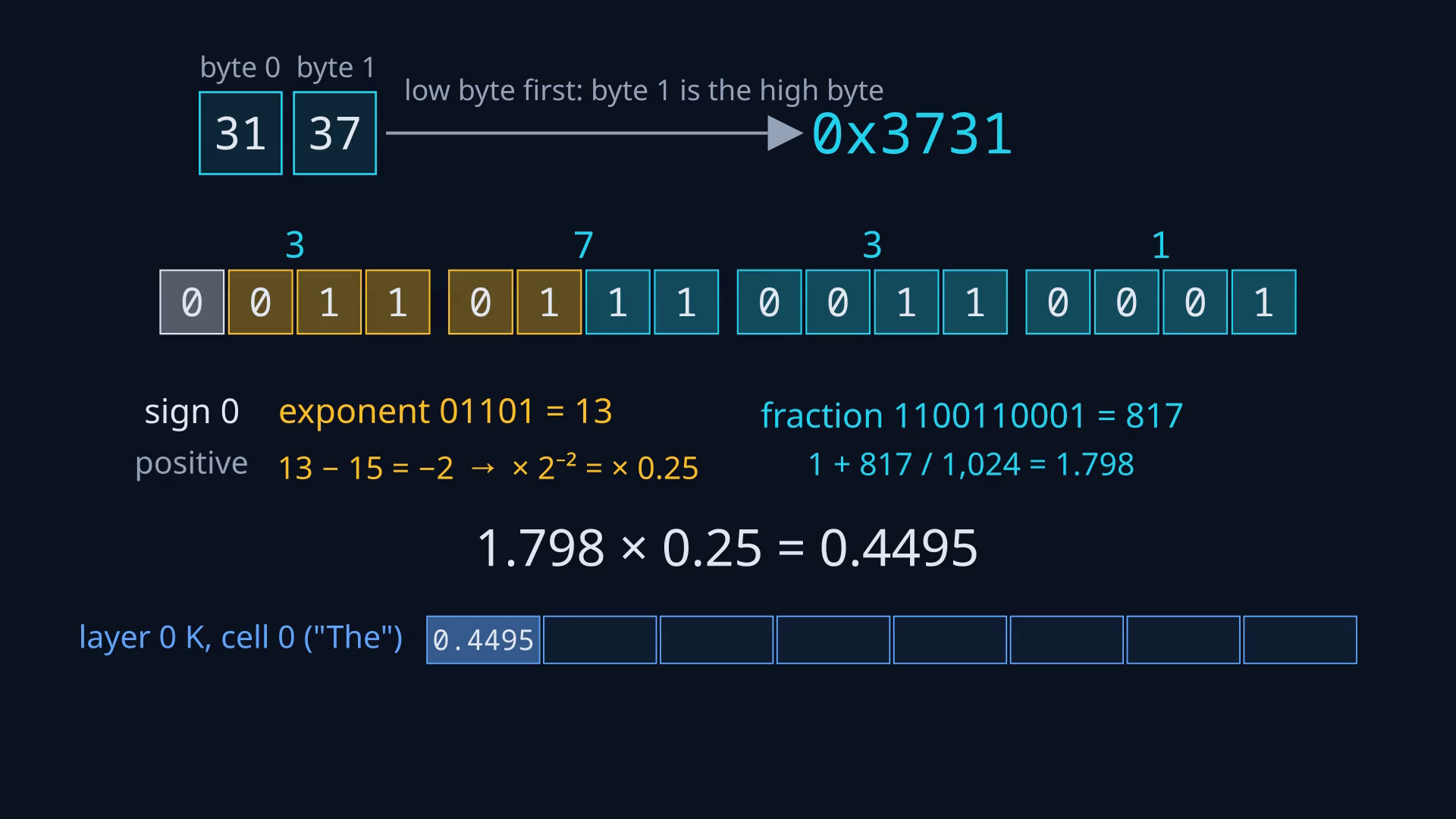
The first two bytes, 31 37, are the little-endian F16 representation of approximately 0.4495. That is an actual cached key value, not an illustrative number.

Bytes 31 37 form F16 bit pattern 0x3731. Its sign, exponent and fraction decode to approximately 0.4495. — Two bytes from the file, decoded into one number.

The dump, full parsed output, probe source, build helper, and parser are available alongside this post. The probe uses a CUDA build of the pinned llama.cpp revision linked below; the parser needs NumPy. Set LLAMA_DIR to that checkout when using the build helper.

The tensor’s three dimensions

A layer’s K tensor has this shape, in ggml’s fastest-dimension-first notation:

[values per token, cells per stream, number of streams]

For this run, that is [1024, 4096, 1]. The row count is capacity, including empty cells. With F16 and Flash Attention enabled, V uses the same layout.

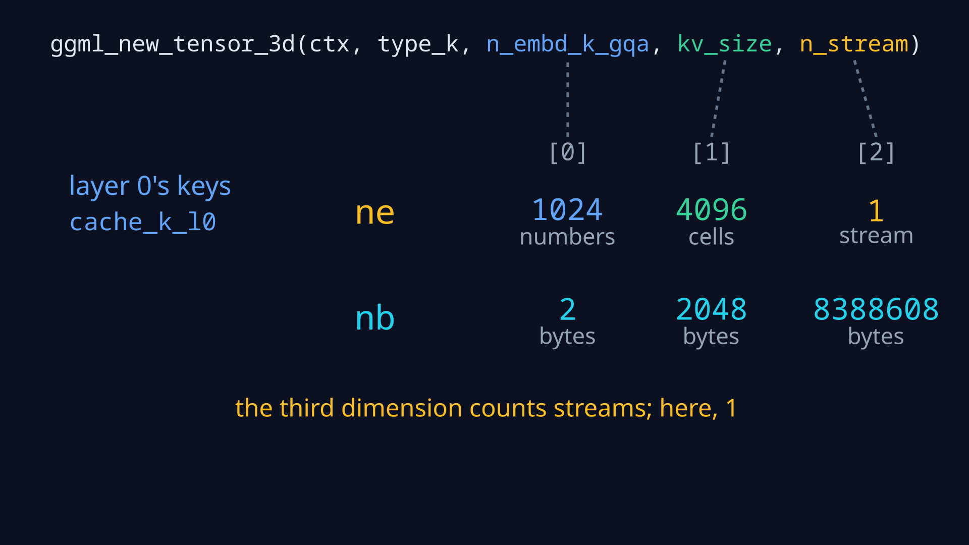
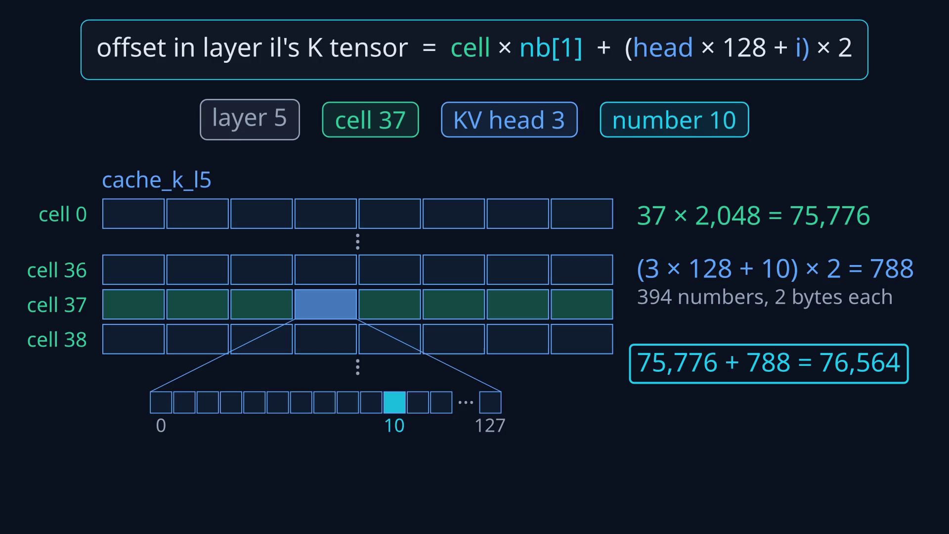
The K tensor has ne dimensions 1024, 4096, 1 and nb byte strides 2, 2048, 8388608. — `ne` gives the sizes. `nb` gives the byte strides: two bytes per number, 2,048 per row, and 8 MiB per stream's slab.

Those strides tell us where any value lives. For example, take layer 5, cell 37, KV head 3, and element 10 within that head. Counting from zero, its offset from the start of that layer’s K tensor is:

37 × 2048 + (3 × 128 + 10) × 2 = 76,564 bytes

Find cell 37's row, then head 3, then element 10. The row offset and in-row offset sum to 76564 bytes. — A row, a head within that row, and one F16 value. This is a tensor-relative address calculation, separate from the seven-token file's offsets.

Unified versus non-unified

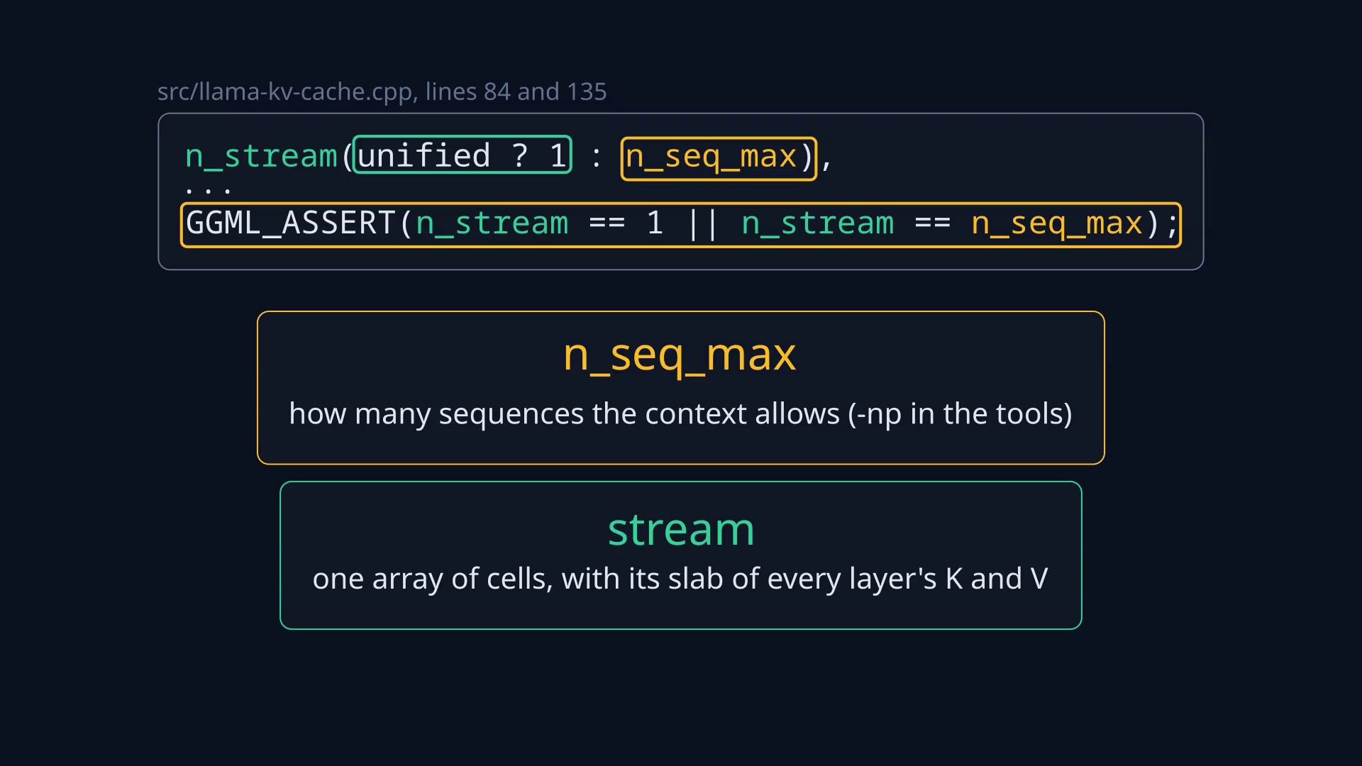
I also dug into how unified and non-unified caches affect that third dimension. Here, a stream means a cache partition, not a CUDA execution stream. A sequence is one independent conversation or run of tokens.

With a unified cache, n_stream is one. Tokens from different sequences occupy rows in the same pool, with bookkeeping and attention masks keeping track of which sequence may read which cells.

With a non-unified cache, n_stream is the maximum number of sequences. Each stream gets a two-dimensional slab of every layer’s K tensor and V tensor. These are views into the larger tensors, not extra copies.

A layer's K tensor contains one two-dimensional slab per stream. ggml_view_2d selects a slab at offset s times nb[2] without copying it. — Each stream occupies one slab. Stream `s` starts at `s × nb[2]`.

The source expresses the choice directly:

n_stream(unified ? 1 : n_seq_max)

And it creates each K slab’s view with:

ggml_view_2d(ctx, k, n_embd_k_gqa, kv_size,
             k->nb[1], s * k->nb[2]);

The stream-selection code

The constructor selects one stream for unified mode or n_seq_max streams otherwise. — With only one allowed sequence, both choices give one stream. The dump above used that single-sequence case.

For a total capacity of 4,096 cells and four sequences, the shapes are:

Mode	K tensor shape, per layer
Unified	`[1024, 4096, 1]`
Non-unified	`[1024, 1024, 4]`

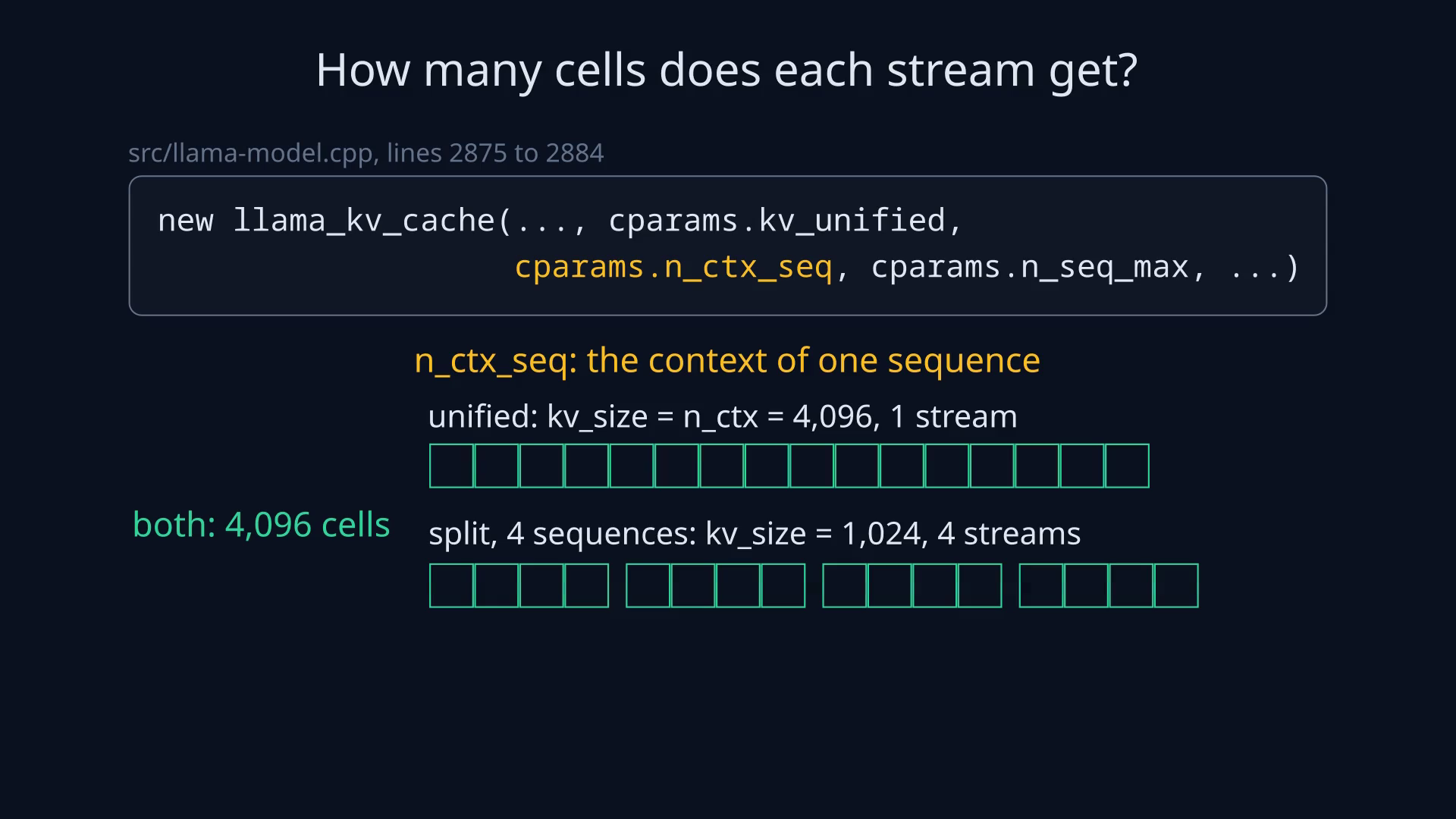
Unified mode has one pool of 4096 cells; non-unified with four sequences has four pools of 1024 cells. Both contain 4096 cells in total. — Same total capacity, different partitioning. Both layouts reserve 448 MiB for this example.

That partitioning explains the speed-versus-memory-efficiency tradeoff. Non-unified attention can read a sequence’s own slice without scanning cells belonging to other sequences, which can make independent concurrent sequences faster. But spare capacity in one stream cannot simply be used by another, and common prefixes need separate copies. Unified keeps a shared pool, making it easier to use the space when conversation lengths differ.

For me, the cache became much easier to picture once I could connect the pieces: 28 pairs of tensors, rows of 1,024 numbers, two bytes per number, and one more dimension deciding how the rows are shared.

Source

The experiment and diagrams use llama.cpp 99b95488c and Qwen3-0.6B. The main code is in llama-kv-cache.cpp, including tensor construction and state serialization.