Weight tying, part 3: what it costs and when to stop

This is the last of three posts on weight tying. Part 1 covered what wte and lm_head do and why their shapes match. Part 2 covered why one matrix can serve both ends without contradiction.

This post is the engineering question: what does sharing actually cost, and why do large models stop doing it?

The answer starts in the backward pass, because that is where the two roles stop being an abstraction and start pulling on the same numbers.

Every number below is printed from the real GPT-2 124M weights.

Two gradients into one tensor, added not broadcast

Because one tensor is used in two places in the forward pass, the backward pass produces two gradients for it, and they are added:

dL/dW  =  (dL/dW via lm_head)  +  (dL/dW via wte)

This is the multivariable chain rule: when a variable affects the loss through several routes, the total derivative is the sum along each route. PyTorch does it with += into .grad, the same accumulation that makes zero_grad() necessary between steps.

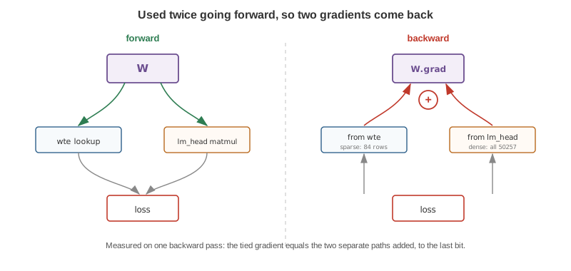
To confirm it, I ran one backward pass on a tied model and on an identical untied copy, so the two contributions could be looked at separately:

tied gradient == (from lm_head) + (from wte)   ->  True,  maxdiff 0.0

Exactly equal, not approximately.

The two routes are very different lengths

Calling them “two gradients” makes them sound symmetric. They are not, and the asymmetry is geometric: the two routes back from the loss have wildly different lengths.

The first route is short. The loss is computed directly from the logits, the logits are x @ W.T, so W is one matmul away from the loss. The gradient arrives after a single step, with nothing in between to attenuate it.

The second route is the whole network. To reach W in its input role, the gradient has to leave the loss, pass back through lm_head, then ln_f, then all twelve transformer blocks in reverse, through every attention and MLP inside them, and only then arrive at the embedding lookup at the bottom. It is the longest path in the model.

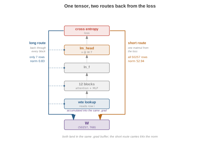
So the same tensor is reached twice in one backward pass, once immediately and once at the very end. Measuring both on "The sky is blue and the grass is green", nine tokens:

short route (lm_head)    rows touched  50257    norm  52.94
long route  (wte)        rows touched      7    norm   0.83

The short route is 64 times larger in norm and touches the entire vocabulary. The long route touches seven rows, one per distinct token in the batch, and arrives small.

Two separate things cause that gap, and they are worth keeping apart. The row count is structural: the output path scores every row at every position, so every row gets a gradient, while the input path only touches rows whose token actually appeared. The magnitude is the journey. Watching the activation gradient on its way down the stack:

leaving block 12    0.060
leaving block  8    0.092
leaving block  4    0.116
leaving block  1    0.086

It stays the same order of magnitude the whole way, which is what residual connections and layer norm are for, but it is already small when it leaves the top and it never grows. The short route never has to make that trip.

One detail I liked. Per-row, the two routes disagree about which tokens matter:

          short route    long route
" grass"       26.29          0.16
" blue"        24.39          0.24
"The"           0.01          0.49
" green"       15.95          0.00

"The" is barely touched by the output path, because it is the first token and almost never the right answer anywhere in this sentence, yet it gets one of the largest input-path gradients, because everything downstream was conditioned on it. " green" is the reverse and its long-path gradient is exactly zero: it is the last token, nothing is predicted after it, so no loss term depends on its embedding at all.

That is the concrete version of the two jobs. One route asks how good a row was as an answer, and it asks about every row. The other asks how good a row was as a starting point, and it can only ask about rows that were actually used.

This also explains a natural guess, that the gradient should be broadcast rather than summed. Broadcasting stretches a smaller shape to fit a larger one, and there is nothing to stretch here: both contributions are already (50257, 768), one value per weight. Addition is the only thing that applies.

The two gradients pull the same row different ways

Adding them is the mechanism, and the two routes explain the reach. The consequence is that the two paths want different things from the same row.

The input path wants row i to be a good starting representation of token i. The output path wants row i to be a good detector, scoring high when token i should come next. On a larger batch than the nine-token sentence used above, comparing the two contributions on the rows they both touch:

rows touched:  input path 84,  output path all 50257
cosine between the two, mean   -0.0069   sd 0.0463
share of rows with negative cosine   54.8%
per-row norm:  lm_head 2.004,  wte 0.025

I want to be careful here, because the tempting reading is wrong. A mean cosine of -0.0069 sounds like the two forces oppose each other. They do not. In 768 dimensions two unrelated vectors have an expected cosine of 0 with a standard deviation of about 1/sqrt(768), or 0.036, so a mean of -0.007 across 84 rows sits about 1.4 standard errors from zero. Pairing each row’s output gradient with a different row’s input gradient, which destroys any real relationship, gives -0.0083 and 58% negative. The shuffled control reproduces the effect, so the effect is not evidence of opposition.

What the numbers do support is weaker, and still worth knowing: the two contributions are close to orthogonal. They are not fighting and they are not cooperating. They push the row in unrelated directions, and their sizes are wildly different, with the output path around 80 times larger per row.

The optimizer never sees the two separately. By the time it runs there is one gradient tensor holding one number per weight, so the row moves along the sum. Given the 80x size gap, that sum is dominated by the output path on almost every row, and the input path acts as a small persistent nudge rather than an equal partner.

The reach of the two paths is very different, and that is the part I found most interesting. In that step the input path touched 84 rows, the ones whose token ids appeared in the batch. The output path touched all 50257, because every row gets scored at every position and so gets told whether it was the right answer.

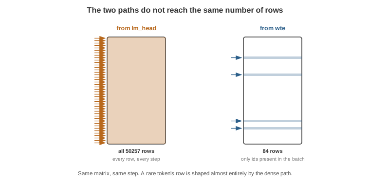
So a rare token’s row is shaped mostly by the output path repeatedly telling it “you were not the answer”, and only occasionally by the input path telling it what it means. Tying is what gives that row a steady signal at all. Untied, its embedding would sit nearly still between the rare times its token shows up.

What tying costs and what it saves

The saving is the obvious argument, and for GPT-2 124M it is a big one. Those 38.6M shared parameters are 31% of the whole model. But that fraction is not a constant, and this is the part that decides whether anyone still ties today.

The embedding table is vocab x d_model, which grows linearly in d_model. The blocks are roughly 12 x d_model^2 each and there are more of them as models get deeper, so the body grows quadratically. Same vocabulary, four GPT-2 sizes:

124M   d= 768  L=12    embedding  38.6M   31.0% of the model
355M   d=1024  L=24    embedding  51.5M   14.5%
774M   d=1280  L=36    embedding  64.3M    8.3%
1.5B   d=1600  L=48    embedding  80.4M    5.2%

The table barely doubles while the model grows twelve times. So tying is a large saving in a small model and a rounding error in a large one, which is exactly what current practice reflects. Qwen3 ties through 4B and stops:

Qwen3-0.6B   tie_word_embeddings = True     embedding ~31% of params
Qwen3-1.7B   tie_word_embeddings = True     ~18%
Qwen3-4B     tie_word_embeddings = True     ~12%
Qwen3-8B     tie_word_embeddings = False    ~8%
Qwen3-14B    tie_word_embeddings = False
Qwen3-32B    tie_word_embeddings = False

Llama draws the line in the same place, independently:

Llama-3.2-1B   d=2048  tie_word_embeddings = True
Llama-3.2-3B   d=3072  tie_word_embeddings = True
Llama-3.1-8B   d=4096  tie_word_embeddings = False

The cut sits where the saving stops being worth the constraint. That is the cost side: tying is a constraint. Two matrices that could have specialized are forced to be one, and the row has to serve both jobs at once, which is the tug of war measured earlier in this post. A big model has the capacity to spend on letting them specialize, and buys back accuracy by doing so. A small model does not, and the constraint is cheap.

Where regularization comes into it

The word regularization gets attached to tying a lot, and it is worth being precise about what is being claimed, because it is not obvious that halving a parameter count has anything to do with overfitting.

A regularizer is anything that makes a model fit its training data less well in exchange for generalizing better. Weight decay does it by penalizing large weights, dropout by deleting activations at random. Tying does it by removing the freedom to make the input and output vectors of a token disagree. It is a hard constraint rather than a penalty, but the effect is the same shape: the model can express fewer functions, so it has fewer ways to memorize.

The reason to believe it is not the parameter count, it is the direction the two error numbers move. Press and Wolf report both, on a large LSTM that already had Bayesian dropout:

                        params    train ppl    test ppl
untied                   66M         37.8        78.4
tied                     51M         48.5        73.2

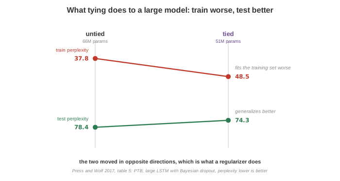
Training perplexity got substantially worse, from 37.8 to 48.5. Test perplexity got better. That opposite movement is the signature of a regularizer, and it is the thing a pure compression argument cannot produce. If tying were only making the model smaller you would expect both numbers to worsen together. Instead the model lost some ability to memorize the training set and gained on text it had not seen.

The mechanism is the one from the tug of war. Untied, the output row for a token is free to become a pure next-token detector, tuned to whatever quirks of the training corpus improve the score. Tied, that same row also has to work as the input representation of the token, so it cannot drift to a corpus-specific position without damaging its other job. The input path acts as an anchor. That is a constraint on where the row can sit, which is what regularization is.

There is a limit to how far to push this. Press and Wolf’s own results show the effect is largest when the model is otherwise unregularized, and their projection regularization trick “does not help the large models, which employ dropout for regularization”. Tying still helped in their dropout models, but it is one pressure among several, not a substitute for dropout. And the modern picture is mostly about the parameter share above: nobody unties a 0.6B model to get regularization back, and nobody keeps a 32B model tied for it either.

Summary of the series

Weight tying sets wte.weight and lm_head.weight to one tensor. It is legal because nn.Linear stores its weight as (out_features, in_features), so both want (50257, 768) and the transpose happens at call time as a view.

It is sensible because the matrix is a set of 50257 token vectors, and the two uses are just two things you can do with such a set: index one out, or score all of them against a query. Cross entropy pushes the vector that predicts a token and the vector that represents it to the same place, so the two jobs turn out to be one constraint applied from both ends.

It has a real cost. The tensor is reached by two backward routes of very different length, one matmul from the loss and the full depth of the network, and they arrive with wildly different sizes. The row settles under whatever the sum does, which is dominated by the output path.

And the decision to use it is mostly about size. The embedding table is 31% of GPT-2 124M and 5% of GPT-2 1.5B, so the saving evaporates as models grow. Both Qwen3 and Llama tie their small models and untie from 8B.

The code here is from llm.c master as of August 2026, mainly train_gpt2.py. Tensors were printed from the pretrained GPT-2 124M weights with PyTorch 2.11 and the gpt2 tokenizer from Hugging Face. If something here is wrong I would like to know.