Backprop: Easy Gradient Shortcut Through Cross-Entropy

Context: This is part 5 in a series that comes out of Andrej Karpathy’s Becoming a Backprop Ninja, where you hand-write every backward pass instead of calling .backward(). Part 1, part 2, part 3 and part 4 worked through individual operations. This one is Exercise 2 from the notebook.

▶ Building makemore Part 4: Becoming a Backprop Ninja, Andrej Karpathy

Cross-entropy is how a classifier turns its raw output into a single number saying how wrong it was. The network’s last layer produces one score, a logit, for every character it could predict next. Softmax turns those scores into probabilities that sum to 1. Cross-entropy then picks out the probability the model gave to the character that actually came next, and takes the negative log of it. Confident and right gives a loss near zero, and the less probability the model left for the right answer, the larger the loss. Averaging that over the batch gives the final loss to be minimized.

In this post, we will look at the cross-entropy layer which is used to calculate the loss.

Here is that calculation written out the long way, broken into its smallest atomic pieces, which is how the earlier posts worked through it. Eight lines, eight intermediate tensors, every one of which needed its own backward pass:

logit_maxes = logits.max(1, keepdim=True).values
norm_logits = logits - logit_maxes    # subtract max for numerical stability
counts = norm_logits.exp()
counts_sum = counts.sum(1, keepdims=True)
counts_sum_inv = counts_sum**-1
probs = counts * counts_sum_inv
logprobs = probs.log()
loss = -logprobs[range(n), Yb].mean()

And here is the whole thing in PyTorch:

loss_fast = F.cross_entropy(logits, Yb)

The interesting part is not that the forward pass collapses. It is that the backward pass collapses too, from five separate gradient computations down to this:

dlogits = F.softmax(logits, 1)
dlogits[range(n), Yb] -= 1
dlogits /= n

Three lines. The middle one is the odd-looking one: it subtracts 1 from a specific set of positions in the matrix. The rest of this post works out where each of the three comes from.

The block we are differentiating

Cross-entropy takes two inputs and returns one number.

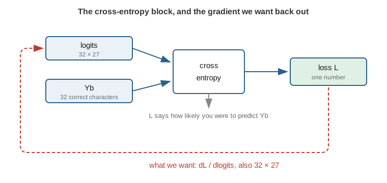
It takes logits, the raw scores the network produced, and Yb, the characters that should actually have come next. It returns $L$, one number measuring how likely the model was to predict Yb. Low probability on the right answer gives a high loss.

What we want back out is $\partial L / \partial\, \texttt{logits}$, which has to be the same shape as logits, because a gradient always has the same shape as the thing it is the gradient of.

Shapes

The logits matrix is 32 rows by 27 columns.

The 32 is the batch size, one row per example. The 27 is the number of output neurons, one per character in the vocabulary: 26 letters plus the . token that marks the start and end of a name.

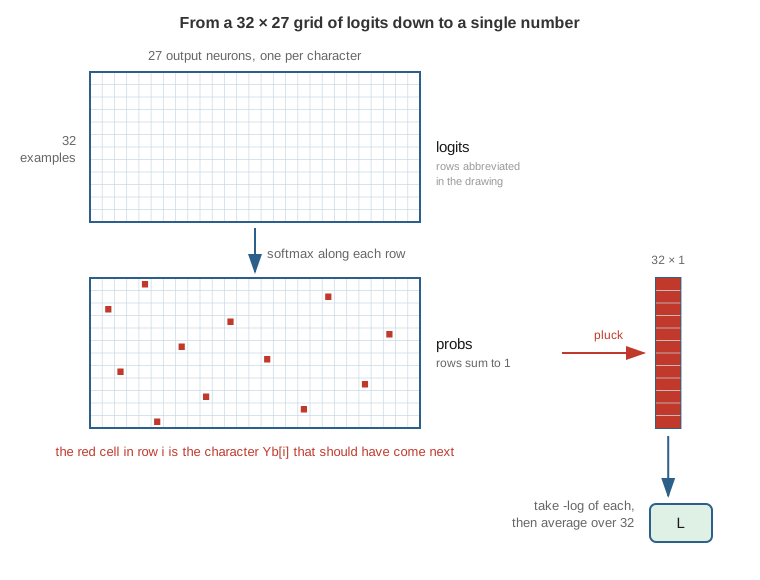
Four things happen, in order:

1. Softmax along each row. Each row of 27 raw scores becomes 27 probabilities that sum to 1.
2. Pluck one probability per row. Yb[i] says which column is the correct character for row $i$, so we take probs[i, Yb[i]]. That gives a column of 32 numbers.
3. Take the negative log of each.
4. Average over the batch.

Written as one expression, with $p_i$ the probability the model gave to the correct character for example $i$:

Which in code is exactly what that last line of the long forward pass said:

loss = -logprobs[range(n), Yb].mean()

Step 2 is worth noting. Out of $32 \times 27 = 864$ numbers in the probability matrix, the loss looks at exactly 32 of them, one per row. The other 832 are never read. That fact does not mean their gradients are zero, as we will see, but it does mean the loss expression itself is a lot smaller than the matrix suggests.

Why the negative log

The loss for a single example is $-\log p$, where $p$ is the probability the model assigned to the correct character. That choice is doing something specific:

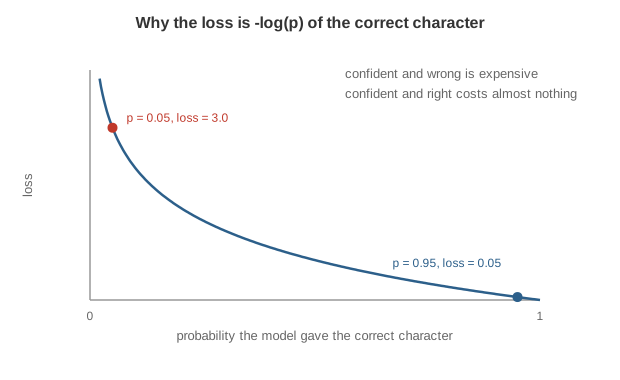
If the model gave the right answer a probability near 1, $\log p$ is near 0 and the loss is near 0. If it gave the right answer a probability near 0, $\log p$ heads for minus infinity and the loss becomes large.

Probabilities live between 0 and 1, so their logs are always negative. The minus sign out front just flips that back to a positive loss.

Two things to notice before any calculus

Both of these make the derivation smaller.

Rows are independent. Row $i$ of the loss depends only on row $i$ of the logits. Softmax runs along a row, and the plucked probability comes from that same row. Nothing crosses between examples. So we can derive the gradient for one row, and then apply the identical formula to all 32.

The $1/n$ is a constant. The batch loss is the mean, so there is a factor of $1/n$ out front. Constants pass straight through differentiation, so park it, do the interesting work without it, and multiply it back at the very end.

That leaves one question: for a single row, what is the derivative of the loss with respect to one logit in that row?

The trick: freeze everything except one

Write the softmax for a single row. Call the logit we are differentiating with respect to $a$. The softmax denominator is a sum over all 27 exponentials:

We are differentiating with respect to $a$ and nothing else. Every other logit in that row is being held fixed. So every other exponential in that denominator is a constant. $e^b$, $e^c$, $e^d$ and the rest genuinely do not change when $a$ changes.

Give the whole pile of them one name, $k$:

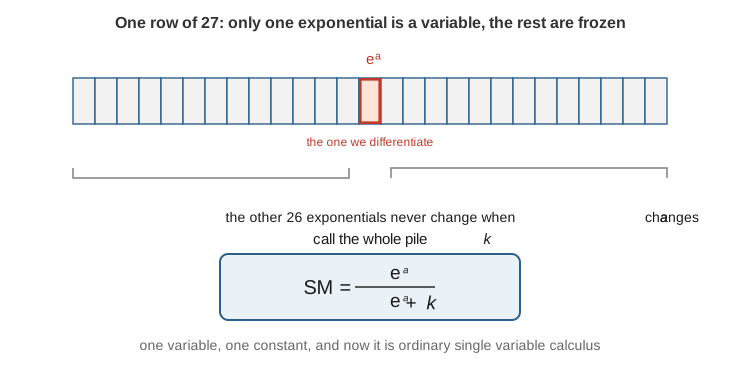
One variable, one constant. The 27-variable problem is now a single-variable one, which you can do by hand or hand to Wolfram Alpha.

One rearrangement will be useful shortly. Since $SM = e^a / (e^a + k)$, we can solve for the denominator and then for $k$ itself:

We will use that in a moment.

Two cases, and why there are exactly two

We need $\partial L / \partial a$ for every logit in the row, all 27 of them, not just the correct one. And the loss expression looks different depending on whether $a$ happens to be the correct character or not.

The loss only ever looks at the probability of the correct character:

Now ask where a given logit $a$ appears in that expression.

• If $a$ is the correct character, then $e^a$ appears twice: once in the numerator, and once inside the denominator sum.
• If $a$ is not the correct character, then $e^a$ appears exactly once, and only in the denominator.

The second case is the less obvious one. A wrong character’s logit still affects the loss, even though the loss never looks at its probability. It affects the loss because it is part of the normalizing sum. Raise a wrong logit and you inflate the denominator, which shrinks the correct character’s probability, which raises the loss. The influence is entirely indirect, routed through the denominator.

That is why the numerator is a constant in the second case. The numerator is the correct character’s exponential, which does not contain $a$ at all, so we can fold it into $k$ as well and write both cases with the same two symbols:

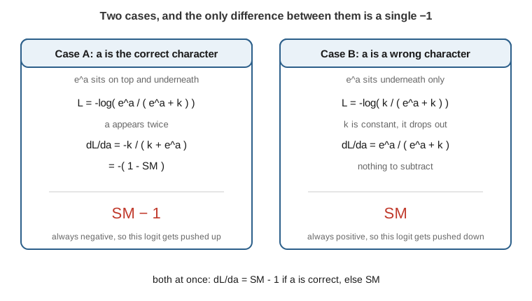
Case A: $a$ is the correct character

The loss for this row, in terms of $a$ and $k$:

Differentiating with respect to $a$ (this is the expression I put through Wolfram Alpha):

Now substitute $k = e^a / SM - e^a$ from earlier:

Multiply top and bottom by $SM / e^a$:

The gradient on the correct character’s logit is its own softmax probability, minus one.

Case B: $a$ is a wrong character

Now $e^a$ only appears in the denominator, and the numerator is the constant $k$:

Again through Wolfram Alpha:

Which is the softmax probability of $a$, with nothing subtracted. Wolfram also gives the equivalent form $1 - k/(k + e^a)$, which is a nice mirror of Case A.

Merging the two cases

Put them side by side:

The $SM$ term is common to both. The only difference is a $-1$ that shows up exactly on the correct character’s position. So write it as one expression, using an indicator that is 1 when $a$ is the correct character and 0 otherwise:

And now bring back the $1/n$ we parked earlier, since the batch loss is a mean over $n$ examples:

Which is exactly the three lines of code, in the same order:

dlogits = F.softmax(logits, 1)     # the SM term, for all 32 x 27 entries at once
dlogits[range(n), Yb] -= 1         # the -1, only at the correct positions
dlogits /= n                       # the 1/n from the mean

Three lines, three terms. F.softmax(logits, 1) runs the softmax along dimension 1, meaning along each row. [range(n), Yb] is the same fancy indexing that plucked out the probabilities in the forward pass, now used to subtract 1 at those same positions. And the division by $n$ is the gradient flowing back through the mean.

Reading the answer as forces

There is a useful way to read the result, and it is the best part of Karpathy’s explanation.

Take one row of dlogits, multiply it by $n$ to undo the batch scaling, and read each cell not as a number but as a force acting on that logit.

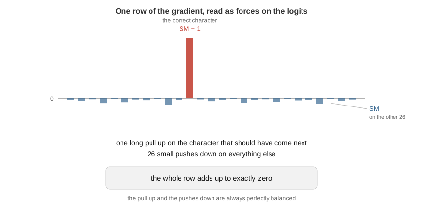
The correct character gets $SM - 1$, which is always negative, since $SM$ is a probability below $1$. Negative gradient means gradient descent will push that logit up. Every wrong character gets $SM$, always positive, so those logits get pushed down.

Now add up the whole row. The probabilities sum to 1, and we subtracted exactly one 1, so:

Every row of dlogits sums to exactly zero. The upward pull on the correct character and the total downward push on the other 26 are always perfectly balanced. The gradient never lifts or lowers a row as a whole, it only moves probability mass around within the row.

Why the signs come out that way

The two formulas, $p - 1$ and $p$, are not arbitrary. Both signs are exactly what you would pick by hand if you were told to reduce the loss and had to choose a direction.

Start from what we actually want. The loss falls when the correct character’s probability goes up. So the correct character’s logit should be increased, and every wrong character’s logit should be decreased, since they compete for the same probability mass through the softmax denominator.

Now recall that gradient descent moves against the gradient:

So a negative gradient increases the parameter, and a positive gradient decreases it. The sign of the gradient is already the instruction for which way to move.

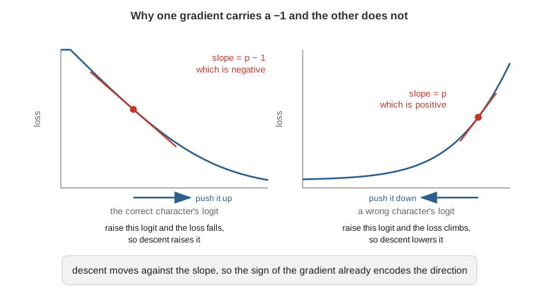
Read the two panels as plots of the loss against a single logit, holding the rest of the row fixed:

• The correct character (left). Raising this logit raises $p$, which lowers the loss, so the curve slopes downward and the tangent has negative slope. That slope is $p - 1$, and since $p < 1$ it is always negative. Descent therefore pushes this logit up, which is what we wanted.
• A wrong character (right). Raising this logit inflates the denominator, which lowers the correct character’s $p$ and raises the loss, so the curve slopes upward. That slope is $p$, always positive. Descent pushes this logit down.

The $-1$ in $p - 1$ is what flips the sign, and it is only present on the correct character. Without it, both cases would be positive and training would push every logit down, including the one that should have won. The indicator is the piece that tells the row which single element is being pulled the other way.

The gradient and the nudge are two different numbers

It is easy to conflate two quantities here, so it is worth separating them explicitly.

The gradient on the correct character is $p - 1$. Since $p$ is a probability in $[0, 1]$, this is a number in $[-1, 0]$. It is negative, or zero when the model is already perfect.

The nudge actually applied to the logit is what descent does with that gradient:

The two minus signs cancel, so the logit moves up by $\eta(1 - p)$. Both of the numbers you might reach for are real, they are just different objects: $p - 1$ is the slope of the loss, and $1 - p$ is the size of the step. The formula in the code is the gradient, $p - 1$.

Here is one row, with $\eta = 0.5$, correct character at index 2:

idx    role       p          gradient     update to logit
0      wrong      0.23882     0.23882        -0.11941
1      wrong      0.05329     0.05329        -0.02664
2      CORRECT    0.39376    -0.60624        +0.30312
3      wrong      0.19553     0.19553        -0.09777
4      wrong      0.11860     0.11860        -0.05930

Only the correct character has a negative gradient, and it is the only one whose logit goes up.

One thing worth ruling out: the expression is $p - 1$, not $-p - 1$. The latter would live in $[-2, -1]$, so it could never reach zero, and a model that already assigns $p = 1$ to the right answer would still get a full-strength shove. That would be wrong. With $p - 1$, a perfect prediction gives a gradient of exactly $0$ and the row is left alone:

p      gradient (p - 1)     step added to logit (1 - p)
0.01        -0.990                    0.990
0.50        -0.500                    0.500
0.90        -0.100                    0.100
0.99        -0.010                    0.010
1.00         0.000                    0.000

The gradient tapering to zero as $p$ approaches 1 is the property that makes this loss behave, and it is only there because the subtracted term is exactly $1$.

The magnitudes are just as deliberate. The size of the push on the correct character is $\lvert p - 1 \rvert = 1 - p$, which is the amount of probability the model failed to put on the right answer:

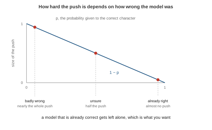
• A confidently wrong prediction, $p$ near 0, gets a push of nearly the full size 1.
• An uncertain prediction, $p$ around 0.5, gets about half that.
• An already correct prediction, $p$ near 1, gets a push near zero. And if $p$ is exactly 1, the gradient at the correct position is $1 - 1 = 0$ and every wrong position holds probability 0, so the entire row is zeros. There is nothing to correct and the update leaves it alone.

So the gradient is self-scaling: the more wrong the model was, the harder the correction, and it tapers to nothing exactly as the model gets it right.

Karpathy’s image for this is a pulley system: you are up at the logits pulling on the correct answer and pushing down the wrong ones, and that tension translates back through the network until it reaches the weights and biases. Each update, the parameters give in to the tug a little.

Verifying it

Checking the result against autograd:

loss_fast = F.cross_entropy(logits, Yb)
print(loss_fast.item(), 'diff:', (loss_fast - loss).item())

dlogits = F.softmax(logits, 1)
dlogits[range(n), Yb] -= 1
dlogits /= n

cmp('logits', dlogits, logits)

The comparison comes back approximate rather than exactly equal, with a maximum difference around $5 \times 10^{-9}$. That is floating point noise, not a mistake in the derivation. The long chain and the short expression are mathematically identical but execute a different sequence of operations, so they round differently in the last bits.

If anything, the short form is the better-behaved one. The eight-line version computes exponentials, sums them, inverts the sum, multiplies, and takes a log, with rounding error accumulating at each step. The three-line version does none of that intermediate work.

Wrapping up

Parts 1 through 4 each took one operation and asked where its inputs showed up in the forward pass. Same question here, applied to the loss itself rather than to a single op.

The shortcut exists for two reasons:

• The loss only touches one column per row. Out of 864 numbers, the loss expression reads only 32 of them. That keeps the expression you have to differentiate small.
• Freezing 26 of the 27 logits turns matrix calculus into ordinary calculus. The $k$ substitution is not an approximation. Those other logits genuinely are constants with respect to the one you are differentiating, and naming them collectively is what reduces the problem to something you can do on paper.

And the result reads the way it does because $p - 1$ is negative and $p$ is positive. Descent moves against the gradient, so those two signs are the instruction “raise the correct one, lower the rest,” with a magnitude that is exactly how much probability ended up in the wrong place.

It is also why frameworks ship cross-entropy as a single fused operation rather than composing it out of a softmax, an index and a log. The fused version has a much shorter backward pass, and this derivation is where that shortness comes from.