Backprop: Propagating Gradient Through a Neuron

Context: Like part 1 and part 2, this comes out of Andrej Karpathy’s Becoming a Backprop Ninja (Part 4 of the spelled-out intro series), where you hand-write every backward pass instead of calling .backward(). These notes are the longer explanation I want on hand the next time I go back to the video. If you have not watched it, start there:

▶ Building makemore Part 4: Becoming a Backprop Ninja, Andrej Karpathy

The first two posts covered single operations. This one covers a linear layer.

N = A @ W + b

The results are dW = A.T @ dN, dA = dN @ W.T, and db = dN.sum(0). The transposes are easy to get backwards from memory. Writing out a small case by hand shows where they come from, which is easier to reconstruct later than the formulas themselves.

The setup

Two inputs, two neurons, and a batch of two samples. The batch size of two matters here, because with a single sample the bias gradient reduces to a copy and the summation is not visible.

A holds the inputs, one row per sample:

A = | a1  a2 |     <- sample 1
    | a3  a4 |     <- sample 2

W holds the weights, where W_ij is the weight from input i into neuron j:

W = | W11  W12 |
    | W21  W22 |

b is one bias per neuron, a single row that gets broadcast down to every sample:

b = [ b1  b2 ]

Multiplying out N = A @ W + b gives a 2x2, one row per sample:

N1 = a1·W11 + a2·W21 + b1        N2 = a1·W12 + a2·W22 + b2      <- sample 1
N3 = a3·W11 + a4·W21 + b1        N4 = a3·W12 + a4·W22 + b2      <- sample 2

Here is that same computation as a picture, with both samples drawn out:

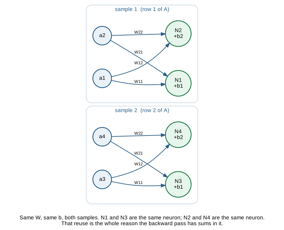
Two things to note from the diagram.

Within a sample, every input reaches every neuron, so a1 is used twice, once per neuron.

Across panels, the two panels are the same layer applied to a second sample, not two different layers. W11 appears in both panels, and so does b1. N1 and N3 are the same neuron with different inputs, as are N2 and N4.

So W and b are shared across samples, while each a belongs to one sample. The rest of the post follows from that.

Backprop gives us the upstream gradient, matching N in shape:

dN = | dN1  dN2 |
     | dN3  dN4 |

and we need to produce dW, dA and db.

Each one comes from the same question used in the earlier posts: where does this variable appear in the output, and how many times?

dW: summing over the batch

Take W11. Search the four expressions above for it. It shows up twice:

• in N1, multiplied by a1
• in N3, multiplied by a3

Two appearances, two paths to the loss, so the chain rule adds them:

dW11 = dN1·a1 + dN3·a3

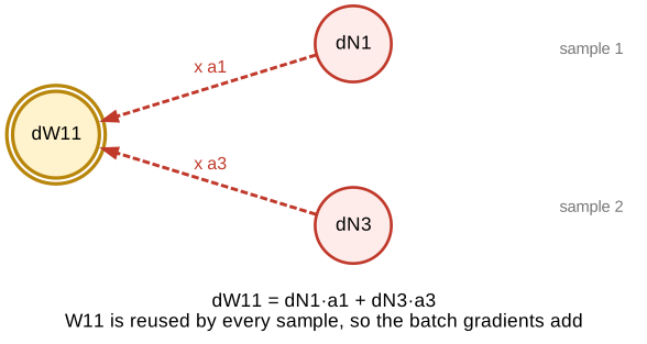
The sum runs over samples. A weight is shared by the whole batch, so each sample contributes a term.

The other three work the same way:

dW11 = dN1·a1 + dN3·a3        dW12 = dN2·a1 + dN4·a3
dW21 = dN1·a2 + dN3·a4        dW22 = dN2·a2 + dN4·a4

Every entry pairs a column of A with a column of dN, summed over the sample index. That is a matrix product with A transposed:

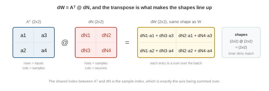
dW = A.T @ dN

A is indexed [sample, input] and dN is indexed [sample, neuron]. Contracting over the shared sample index requires that index on the inside of the product, and transposing A puts it there. The .T is what a sum over the batch looks like in matrix form.

dA: summing over the neurons

Same procedure, different variable. a1 appears in N1 (scaled by W11) and in N2 (scaled by W12). It does not appear in N3 or N4, which belong to sample 2.

da1 = dN1·W11 + dN2·W12

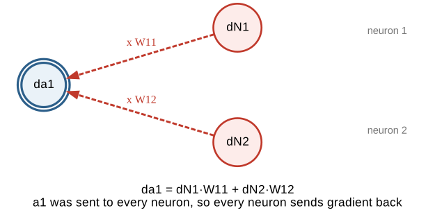
This time the sum runs over neurons rather than samples, because the input was sent to every neuron in the layer.

All four:

da1 = dN1·W11 + dN2·W12        da2 = dN1·W21 + dN2·W22
da3 = dN3·W11 + dN4·W12        da4 = dN3·W21 + dN4·W22

which packs into:

dA = dN @ W.T

The two forms are symmetric, which is a useful way to keep the transposes straight:

• dW = A.T @ dN sums over samples, because a weight is shared across the batch.
• dA = dN @ W.T sums over neurons, because an input is shared across the layer.

Two kinds of sharing, two axes to sum over. The transpose goes wherever it needs to for the shared index to end up on the inside.

db: the bias

b1 is added into N1 and into N3, and it is not scaled by anything, so the local derivative is 1 in both cases:

db1 = dN1·1 + dN3·1 = dN1 + dN3

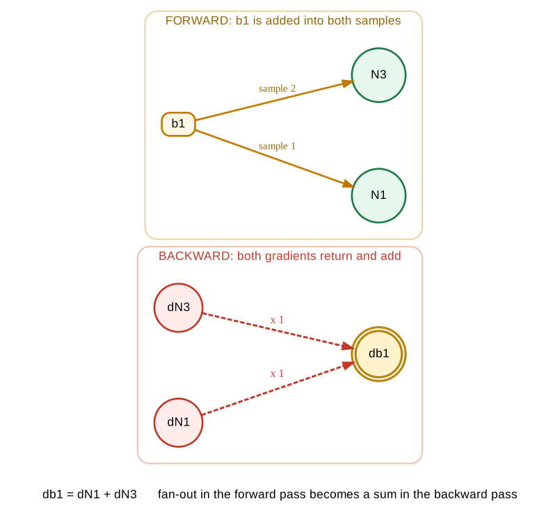
The top panel is the forward pass, where one bias goes out to every sample. The bottom panel is the backward pass, where those arrows reverse and meet at the same node. Two arrows arriving at one node means the values add.

Both biases:

db1 = dN1 + dN3        db2 = dN2 + dN4

which is a column-wise sum, collapsing the batch dimension:

db = dN.sum(axis=0, keepdims=True)     # shape (1, 2)

This is the same rule as part 1. Writing + b broadcasts a (1, 2) row down to (2, 2), broadcasting is a copy, and copies backprop as sums. The only difference from part 1 is the axis: there the broadcast ran across columns, here it runs down rows.

There is no .T in db and no weight either. The bias is added rather than multiplied, so nothing scales its gradient on the way back.

Shape checking

The shape check from the earlier posts is useful here, because it settles the transposes without doing any calculus.

A gradient has the same shape as the thing it differentiates:

A  is (2, 2)  ->  dA  must be (2, 2)
W  is (2, 2)  ->  dW  must be (2, 2)
b  is (1, 2)  ->  db  must be (1, 2)
dN is (2, 2)

The 2x2 case hides this since everything is square. With a batch of 32 samples, 784 inputs and 100 neurons:

A  (32, 784)      W  (784, 100)      b  (1, 100)      dN  (32, 100)

only one arrangement works for each:

• dW must be (784, 100). From A (32, 784) and dN (32, 100), the product that fits is A.T @ dN, which is (784, 32) @ (32, 100).
• dA must be (32, 784). The fit is dN @ W.T, which is (32, 100) @ (100, 784).
• db must be (1, 100). From dN (32, 100), the 32 has to go, so sum over axis 0.

All three can be reconstructed from the shapes alone.

Verifying it

import torch

A = torch.randn(2, 2, requires_grad=True)
W = torch.randn(2, 2, requires_grad=True)
b = torch.randn(1, 2, requires_grad=True)

N = A @ W + b
dN = torch.randn(2, 2)
N.backward(dN)

print(torch.allclose(W.grad, A.T @ dN))                    # True
print(torch.allclose(A.grad, dN @ W.T))                    # True
print(torch.allclose(b.grad, dN.sum(dim=0, keepdim=True))) # True

Summary of the series

All three posts come down to counting how many times a variable is used in the forward pass:

• Used once: the gradient passes straight through. That was A in the subtraction from part 1.
• Used many times: the gradient is a sum, one term per use. That is the bias here, the broadcast vector in part 1, and every weight in a batched layer.
• Used conditionally: gradient flows only on the paths that were taken. That was the max in part 2, where the losing entries got zero.

dW and dA are the second case in matrix notation. The transpose is what a sum over a shared index looks like when written as a matrix product.