Flash Attention, tiled: exact attention without the T x T HBM matrix

Ordinary causal attention has a storage problem before it has a math problem. For a sequence of length T, it forms a T x T score matrix, transforms it into another T x T probability matrix, and then multiplies that by V. Those large intermediates live in GPU high-bandwidth memory, or HBM, which is large but costly to read and write repeatedly.

FlashAttention keeps the same dense-attention result while changing the schedule. It computes small score tiles in fast on-chip memory, updates a little softmax state for each query row, immediately uses the tile’s probabilities to scale value vectors, and avoids materializing the complete T x T score or probability matrix in HBM.

That distinction is the point of this post:

• Ordinary attention: materializes large T x T intermediates in HBM.
• Flash Attention: evaluates the equivalent interactions tile by tile without storing those complete intermediates in HBM.

Exact dense attention still compares T queries with T keys, so its arithmetic remains quadratic in sequence length. Flash Attention is not an approximation and does not make exact dense attention linear-time. It is an IO-aware algorithm: it accounts for data movement between HBM and the much smaller on-chip SRAM and registers.

Contents

1. Ordinary causal attention
2. A three-token example
3. Online softmax, one row at a time
4. What happens when the maximum changes
5. From the example to tiled GPU work
6. More arithmetic can still be faster
7. FlashAttention-2 and the PyTorch call
8. Validation code
9. References

Ordinary causal attention

For one attention head, use these names consistently:

• B is the batch size: the number of independent sequences evaluated together.
• H is the number of attention heads: separate attention calculations running in parallel.
• T is the sequence length: the number of token positions in each sequence.
• d is head_size: the number of components in every query, key, and value vector for one head.
• Q, K, and V are the query, key, and value tensors. Each has shape (B, H, T, d).

For each query row, S names its raw score matrix, P the softmax probability matrix, and Y the final output: a weighted sum of value vectors.

The score matrix for one head is:

S = (Q K^T) / sqrt(d)          shape: T x T

Row i contains one score for every key as seen by query i. In causal attention, query i may use only keys at positions <= i. Scores for future positions are set to negative infinity before softmax, which makes their probabilities zero.

The ordinary PyTorch spelling is:

att = (q @ k.transpose(-2, -1)) * (1.0 / math.sqrt(k.size(-1)))
att = att.masked_fill(mask == 0, float('-inf'))
att = F.softmax(att, dim=-1)
y = att @ v

att is first the score matrix and then the probability matrix. Both have shape (B, H, T, T). The final y has shape (B, H, T, d).

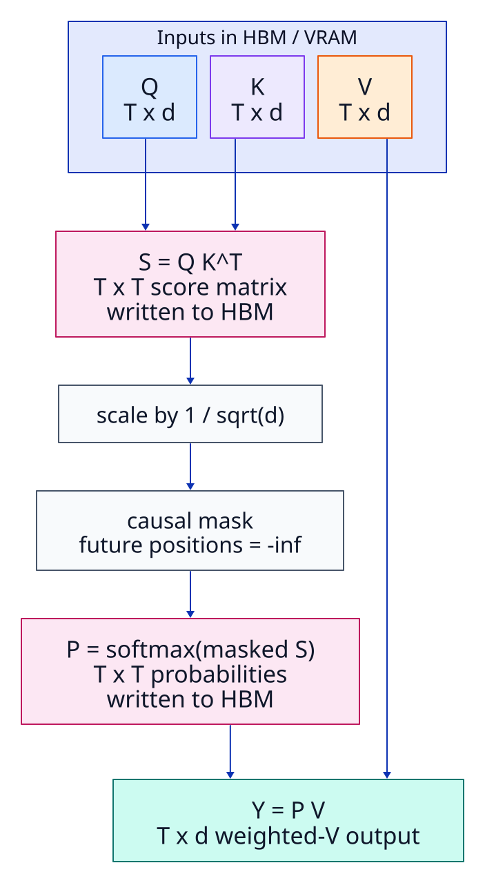
Figure 1. Ordinary attention stores both the score matrix S and probability matrix P in HBM.

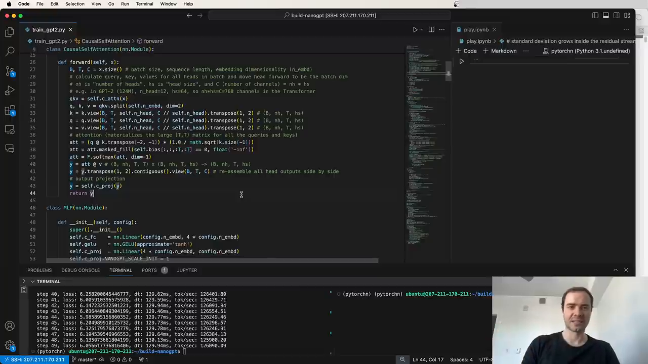
Figure 2. Andrej Karpathy, 2:00:26, with the ordinary multi-operation attention code visible. The screen capture is included for commentary under the video source; the mathematical claims in this post are cited to the primary papers below.

A three-token example

Here is a deliberately small case where the attention arithmetic is visible:

B = 1
H = 1
T = 3
head_size = 2
Q, K, V shape = (1, 1, 3, 2)

The two components in each value vector come from head_size = 2. A probability remains a scalar, but it scales the entire value vector. The small head size is only for readable arithmetic. The GPT-2 124M configuration in Karpathy’s walkthrough code uses 12 heads of size 64, for 768 embedding components.

q = torch.zeros(1, 1, 3, 2)
k = torch.zeros(1, 1, 3, 2)

v = torch.tensor([[[
    [10.0,  0.0],  # V0
    [ 0.0, 20.0],  # V1
    [30.0, 30.0],  # V2
]]])

Because every query and key is zero, every raw dot product is zero:

q @ k.transpose(-2, -1)

[[0, 0, 0],
 [0, 0, 0],
 [0, 0, 0]]

Real query rows do not normally have identical all-zero scores. Here the zeros isolate the causal mask, the softmax denominator, and the value-vector arithmetic.

The causal mask produces:

[[0,   -inf, -inf],
 [0,    0,   -inf],
 [0,    0,    0  ]]

Row-wise softmax produces:

[[1,   0,   0  ],
 [1/2, 1/2, 0  ],
 [1/3, 1/3, 1/3]]

So the ordinary output is:

Y0 = V0                         = [10, 0]
Y1 = (V0 + V1) / 2              = [5, 10]
Y2 = (V0 + V1 + V2) / 3         = [13.333, 16.667]

Online softmax, one row at a time

The original online-normalizer work is Milakov and Gimelshein’s 2018 NVIDIA paper. It maintains a running row maximum and softmax denominator in one pass, with fewer memory accesses than separate maximum and normalization passes.

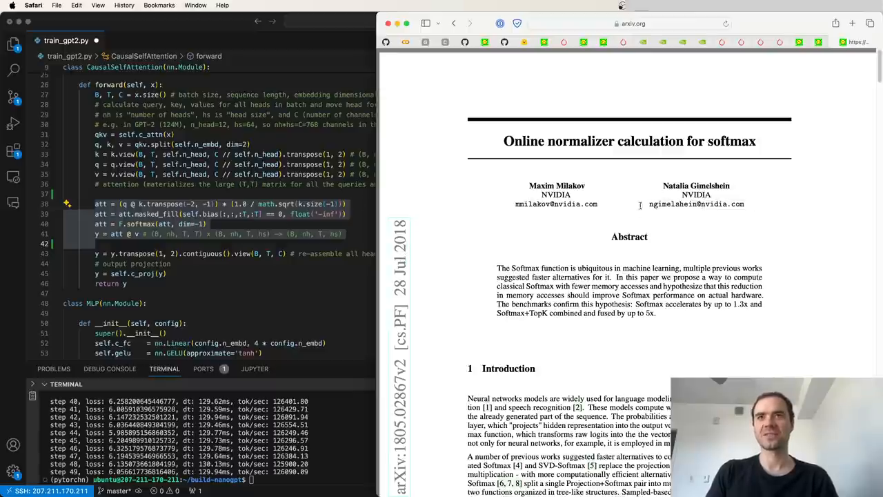
Figure 3. Karpathy, 2:03:50, opening the NVIDIA online-normalizer paper. The recurrence originated there, before FlashAttention used the same kind of running state for tiled attention.

For one query row, maintain three values:

m = largest score seen so far                      scalar
l = sum of exp(score - m) seen so far              scalar, also known as the softmax denominator
o = sum of exp(score - m) * value seen so far      vector of length head_size

output = o / l

Each query row has its own separate m, l, and o. When the explanation moves from row 0 to row 1, it starts a new state. A real kernel updates many rows in a query tile at once, but no row inherits another row’s partial numerator or denominator.

Every permitted score in this teaching example is zero, so every active exponential is simply exp(0) = 1. The three rows below therefore use the direct 1 weights first. The later nonzero example shows why the running maximum m and its correction factor are necessary.

Row 0 starts fresh

Row 0 can see only K0,V0:

m = -inf, l = 0, o = [0, 0]

process score 0:
m = 0
l = 1
o = V0 = [10, 0]

Y0 = o / l = [10, 0]

Row 1 starts fresh

Discard row 0’s state. Row 1 sees K0,V0 and K1,V1:

m = -inf, l = 0, o = [0, 0]

m = 0
l = 1 + 1 = 2
o = 1*V0 + 1*V1 = [10, 20]

Y1 = o / l = [5, 10]

Row 2 starts fresh, then uses two tiles

Discard every other row’s state. Row 2 begins with a fresh state:

m = -inf
l = 0
o = [0, 0]

The first tile has keys and values 0 and 1:

tile 1 scores = [0, 0]

m = 0
l = 1 + 1 = 2
o = 1*V0 + 1*V1 = [10, 20]

The score values and exponential weights for this tile are consumed immediately. They do not need to become row 2 of a full T x T HBM tensor.

The second tile has key and value 2:

tile 2 score = [0]

l = l + 1
  = 2 + 1
   = 3

o = o + V2
   = [10, 20] + [30, 30]
   = [40, 50]

Y2 = o / l = [13.333, 16.667]

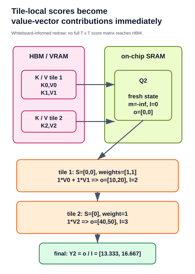
Figure 4. Original redraw informed by the supplied whiteboard. The K and V data arrive as tiles. Each tile’s local softmax weights are multiplied by complete value vectors before the state is updated.

What happens when the maximum changes

The all-zero example has a convenience: the running maximum never changes, so every correction factor is one. The maximum matters when a later tile contains a higher score.

Subtracting a row maximum is safe because the same factor appears in every softmax numerator and denominator:

softmax(si) = exp(si - m) / sum_j exp(sj - m)

The largest exponent becomes exp(0) = 1, avoiding overflow. In online processing, a later tile can change m, so the old partial state must be translated to the new maximum first.

Suppose one query row receives:

tile 1 scores: [1, 2]
tile 2 score:  [4]

After the first tile:

m = 2
l = exp(1 - 2) + exp(2 - 2)
  = exp(-1) + 1

o = exp(-1)*V0 + 1*V1

When score 4 arrives:

m' = 4
r = exp(m - m')
  = exp(2 - 4)
  = exp(-2)

l = r*l + exp(4 - 4)
o = r*o + exp(4 - 4)*V2
m = m'

For a current score tile s and its value tile Vtile, the row-local update can be written as:

m' = max(m, max(s))
r  = exp(m - m')
p  = exp(s - m')

l = r*l + sum(p)
o = r*o + p^T @ Vtile
m = m'

Here p is a vector of scalar weights for the current tile, while Vtile contains full head_size-component value vectors. Therefore p^T @ Vtile is another head_size-component vector, ready to add to o.

From the example to tiled GPU work

A GPU has a memory hierarchy. HBM or VRAM holds large model tensors, but reading and writing it costs more time and energy than operating on data already in the small SRAM and registers close to the compute units.

The FlashAttention paper uses tiles of Q, K, and V that fit in on-chip memory. The pedagogical schedule below holds a query tile and its row-local state on chip while successive K/V tiles are visited. Production kernels can choose a different loop order to fit a particular GPU’s SRAM and work partitioning, but the state update is the same.

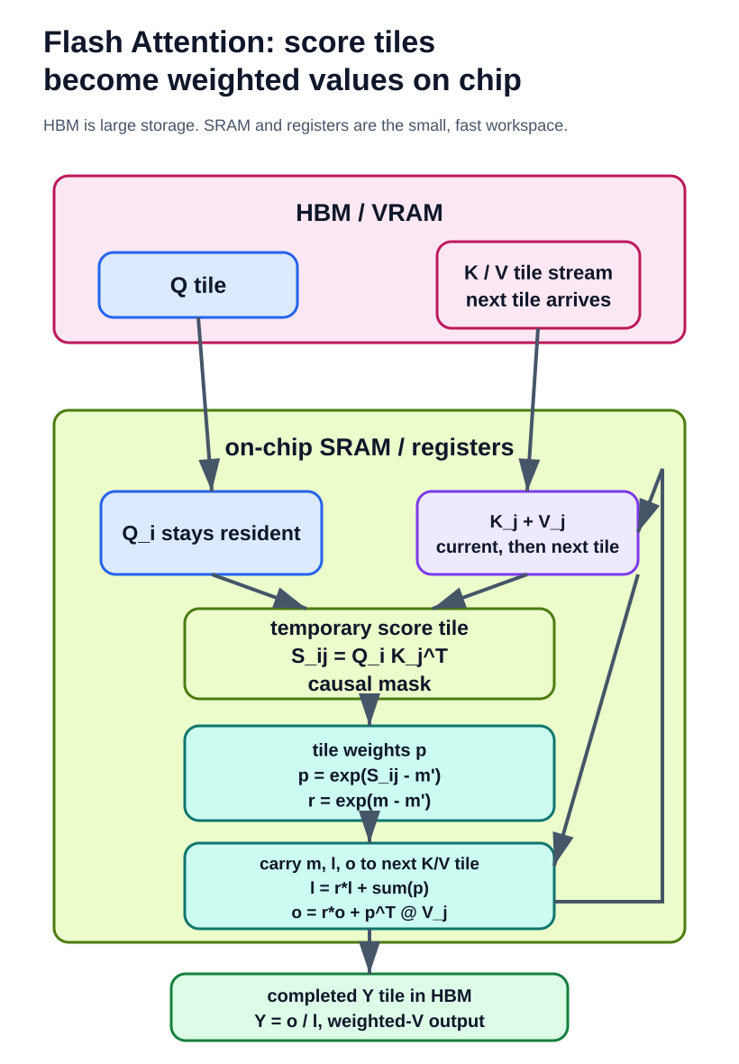
Figure 5. S_ij becomes tile weights p; the kernel immediately forms p^T @ V_j and adds that weighted value vector to o. The row’s m, l, and o carry into the next K/V tile. If the tile finds a larger maximum, r rescales the carried l and o first. After the last tile, Y = o / l is the final weighted-value output written to HBM.

m, l, and o are not reset between K/V tiles. They carry the partial result from one tile to the next. Only after the final K/V tile does the kernel divide o by l to form Y.

Lower-case o is the running, unnormalized weighted-value numerator. Upper-case Y is the final weighted-value output after the division by l.

For one pair of tiles, the kernel performs these operations before moving on:

1. Load relevant Q_i, K_j, and V_j blocks into on-chip memory.
2. Compute local scores S_ij = Q_i @ K_j.T.
3. Apply the causal mask to positions where a query would see a future key.
4. Compute tile exponentials and the per-row maximum and sum.
5. Update every row’s separate (m, l, o) state.
6. Multiply the tile’s probability weights by V_j immediately, adding the resulting value vectors into o.
7. Discard the temporary score and probability tile after its contribution is incorporated.
8. Write the completed output block when all relevant K/V tiles have been processed.

Dao et al.’s FlashAttention paper describes this as an IO-aware exact-attention algorithm. Its forward algorithm computes score tiles, row maxima, exponentials, and value products on chip; it writes the output and limited softmax state rather than the full score and probability matrices.

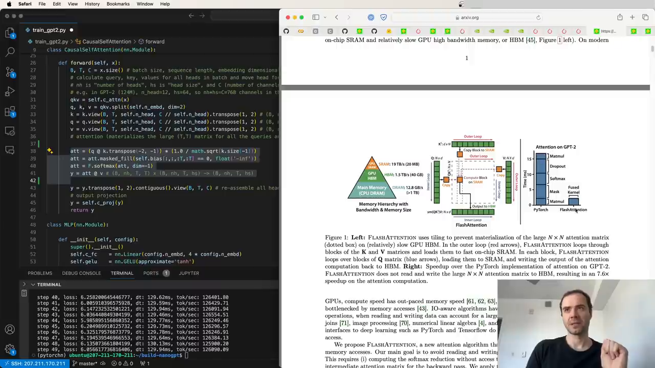
Figure 6. Karpathy, 2:01:13, with Figure 1 of the FlashAttention paper onscreen. The figure connects the memory hierarchy, tiled schedule, and reduced HBM traffic discussed here.

More arithmetic can still be faster

The apparent contradiction is useful: Flash Attention can recompute some quantities and execute more floating-point operations, yet finish sooner.

A matrix multiply is very fast once its operands are near the GPU compute units. Repeated HBM transfers are comparatively expensive. The FlashAttention paper reports that recomputation in the backward pass can raise FLOP count while lowering HBM traffic enough to reduce elapsed time. The implementation trades some arithmetic for much less movement of T x T intermediates.

This is more than ordinary operator fusion. A compiler can fuse adjacent operations when their existing computation graph permits it. The FlashAttention rewrite changes the storage schedule and introduces online state so the full attention matrix is never materialized in HBM. It may also recompute blocks in the backward pass. In Karpathy’s walkthrough around 2:01:13, the contrast is between familiar kernel fusion and this algorithmic change. torch.compile did not infer that new tiled online-softmax algorithm from the straightforward sequence of PyTorch operations in that example.

FlashAttention-2 and the PyTorch call

FlashAttention-2 is a follow-on implementation and algorithm paper, not a renamed contribution of FlashAttention-1. It improves parallelism and work partitioning: it reduces non-matmul work, partitions a single head across thread blocks to increase occupancy, and reduces shared-memory communication between warps. Karpathy transitions to this lineage at about 2:03:26.

At the Python level, the ordinary attention block can be replaced with:

y = F.scaled_dot_product_attention(q, k, v, is_causal=True)

This is not a promise that every call on every machine runs one identical Flash Attention kernel. According to the PyTorch documentation, the operator chooses among supported implementations according to the backend and input constraints. On CUDA it may dispatch an optimized fused kernel, including FlashAttention-2; on other backends or unsupported shapes and data types, it can select another implementation.

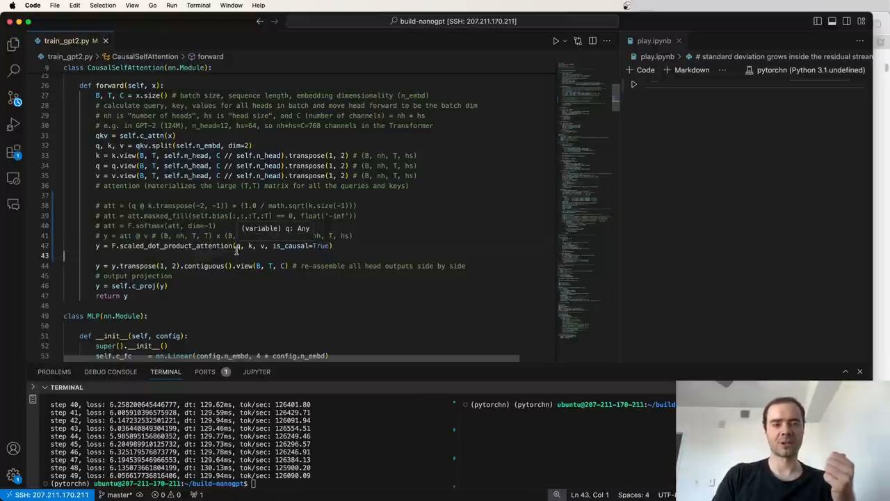
Figure 7. Karpathy, 2:05:20, immediately after the one-line scaled_dot_product_attention replacement is visible in the code.

Validation code

This runnable PyTorch program computes the example two ways: explicitly, and through scaled_dot_product_attention. On a CPU the second call will normally use a math implementation. On a supported CUDA configuration it may choose a fused backend. Either way, both paths implement the same causal attention result.

import torch
import torch.nn.functional as F

q = torch.zeros(1, 1, 3, 2)
k = torch.zeros(1, 1, 3, 2)
v = torch.tensor([[[
    [10.0,  0.0],
    [ 0.0, 20.0],
    [30.0, 30.0],
]]])

scale = q.size(-1) ** -0.5
scores = (q @ k.transpose(-2, -1)) * scale
causal_mask = torch.tril(torch.ones(3, 3, dtype=torch.bool))
scores = scores.masked_fill(~causal_mask, float('-inf'))
probabilities = torch.softmax(scores, dim=-1)
manual_output = probabilities @ v

fused_output = F.scaled_dot_product_attention(
    q, k, v, is_causal=True
)

print(probabilities)
print(manual_output)
print(fused_output)
print(torch.allclose(manual_output, fused_output))

The probabilities are the lower-triangular rows shown above, and the final check is:

True

The core insight

Flash Attention does not remove dense attention’s quadratic arithmetic. It removes a costly habit of the ordinary implementation: writing the full score and probability matrices to HBM and reading them back for the next operation.

Tiling plus online softmax lets each score tile contribute directly to the final value-vector output. The result is exact attention, rearranged around the GPU memory hierarchy.

References

1. Maxim Milakov and Natalia Gimelshein, Online normalizer calculation for softmax, NVIDIA, 2018. PDF.
2. Tri Dao, Daniel Y. Fu, Stefano Ermon, Atri Rudra, and Christopher Re, FlashAttention: Fast and Memory-Efficient Exact Attention with IO-Awareness, 2022. PDF.
3. Tri Dao, FlashAttention-2: Faster Attention with Better Parallelism and Work Partitioning, 2023. PDF.
4. Andrej Karpathy, Let’s reproduce GPT-2 (124M), video walkthrough. Relevant Flash Attention discussion: 2:00:26 through 2:05:20.
5. PyTorch, torch.nn.functional.scaled_dot_product_attention.