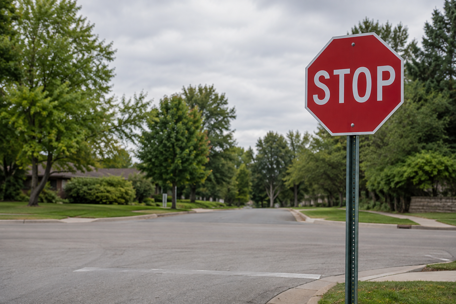
Suppose we train a tiny model to recognize a stop sign. It can use two features:
- color, measuring how red the object is;
- shape, measuring how much it resembles an octagon.
Give each feature a weight and add the results:
\[\text{stop score} = w_c(\text{redness}) + w_s(\text{octagon-ness}).\]The weights describe how strongly those detected features affect the answer. In a neural network the routes are not usually this easy to name, but the basic relationship is the same: a weight controls how much one activation contributes to another.
This example makes a specific point about weight decay concrete:
Weight decay does not force equal distribution. It distributes work only when multiple routes are comparably useful.
Many answers can fit the training data
Start with an intentionally underdetermined training set. Every stop sign in it is perfectly red and perfectly octagonal, so both feature values are 1. The desired score is 2. Training therefore asks only for
\[w_c + w_s = 2.\]There are infinitely many solutions. Here are five:
| Color weight $w_c$ | Shape weight $w_s$ | Training score | Squared weight size $w_c^2+w_s^2$ |
|---|---|---|---|
| 2.0 | 0.0 | 2.0 | 4.0 |
| 1.5 | 0.5 | 2.0 | 2.5 |
| 1.0 | 1.0 | 2.0 | 2.0 |
| 0.5 | 1.5 | 2.0 | 2.5 |
| 0.0 | 2.0 | 2.0 | 4.0 |
The training examples cannot distinguish these outcomes. They all receive the same score and can have the same training loss. Yet they do not behave alike outside that narrow dataset. A color-only solution may mistake a red circular sign for a stop sign. A shape-only solution may be more robust at night or in a grayscale image. Which outcome is good depends on what the features mean and what the model later encounters.
Weight decay adds a preference among otherwise comparable fits: prefer smaller weights. Under the simple constraint above, $(1,1)$ has the smallest squared size. Dividing the work between two equally scaled, interchangeable routes needs less total squared weight than making one route do everything.
That is where distributed work comes from. It is not a command that every feature receive an equal vote. It is the lowest-cost choice in this particular symmetric situation.
The gravity analogy
Karpathy describes weight decay as a kind of gravity pulling weights toward zero. With AdamW, a simplified update is
\[w_{t+1} = (1-\eta\lambda)w_t - \eta\,\text{AdamUpdate}_t,\]where $\eta$ is the learning rate and $\lambda$ is the weight-decay coefficient. The first term is gravity: in the absence of a useful task gradient, the weight becomes a little smaller each step. The second term is the learning signal, which can push a useful weight away from zero.
One way to describe this is that weights must “prove their salt.” There is no separate examination of each weight. A connection remains large only when the training gradients repeatedly provide enough evidence to counter the shrinkage. A route that does not help the prediction receives little opposing pressure and gradually fades.
Take the $(1,1)$ solution and imagine, for clarity, a deliberately large decay step that changes both weights from $1.0$ to $0.99$. For an example whose redness and octagon-ness are both 1, the score falls from 2 to
\[(0.99)(1) + (0.99)(1) = 1.98.\]The prediction loss sees that 1.98 is below the desired score of 2. Its gradient pushes upward on whichever weights help correct the error. Training settles into a tug of war: decay pulls weights toward zero, while the prediction gradient pushes useful weights away from zero. A useless weight feels the pull of decay but receives no consistent push in the other direction.
The change from $1.0$ to $0.99$ is exaggerated to make the arithmetic visible. In the walkthrough, the shrinkage in a single step is much smaller. With a learning rate of $0.0006$ and weight_decay=0.1, the decay multiplier for one simplified step is
So 0.1 does not mean that AdamW removes ten percent of every weight on every step. The per-step effect also depends on the learning rate, and repeated small effects accumulate over training.
When decay spreads the work
Suppose the training set contains both stop signs and other objects. Most stop signs are clearly red and octagonal, and either clue is about equally good at separating the stop signs from the other objects. The model also represents both clues with numbers on roughly the same scale. Because either route can reduce the loss, the task gradient can sustain both. Among solutions with similar training performance, decay favors the one that accomplishes the job with less overall weight magnitude. In the symmetric toy problem, that is the balanced $(1,1)$ solution.
Why this can improve generalization
This can improve robustness because the prediction is no longer resting on one large coefficient when another genuinely useful route is available. More generally, large networks have vastly more parameters than any one training example can constrain. Many parameter settings can fit the observations, but only some behave well on new data. Regularization supplies an extra preference when the loss alone leaves a choice unresolved.
Without decay, the model can give a large weight to an accidental pattern in the training set. Suppose every photographed stop sign happens to have a tree nearby. A tree_nearby feature could then help reduce training loss even though trees will not reliably accompany stop signs in new photographs. Weight decay makes maintaining that extra large weight more costly, which can reduce the model’s reliance on the shortcut.
Decay does not reveal that the tree is irrelevant. If tree_nearby predicts the label perfectly throughout the training data, the prediction gradient may continue supporting it. Weight decay may then be insufficient. Counterexamples, such as stop signs without trees and trees without stop signs, give the model direct evidence that the shortcut does not generalize.
It still does not guarantee the solution that works best on new examples. Weight decay prefers smaller weights. It does not understand what the model’s feature activations represent or whether those features will remain useful on new examples.
When decay should not spread the work equally
Now suppose the training set contains objects with many different shapes, while redness reliably predicts the target:
- redness is predictive;
- shape is mostly noise.
The gradient from prediction errors repeatedly pushes $w_c$, the color weight, upward. It does not consistently push $w_s$, the shape weight, in either direction. Decay pulls both weights downward, but only the color weight receives a repeated push back. A sensible result might look like
\[w_c=1.7, \qquad w_s=0.2,\]not $(1,1)$. Weight decay has not failed. Equal distribution was never its rule.
When regularization hurts
Useful weights also feel gravity. If the decay coefficient is too strong, the task gradient cannot maintain the magnitude required to fit even the real pattern. The model underfits.
Consider night images where color carries almost no information and recognizing the shape requires a strong coefficient. Pulling that coefficient down simply to make the parameter vector small worsens both training and validation performance. Regularization is a tradeoff, not a free improvement.
Feature scaling matters too. If “redness” is numerically 100 times smaller than “octagon-ness,” it needs a larger coefficient to have the same effect. A penalty on coefficient size then treats the two routes differently even if their information content is identical. The balanced solution in parameter space is not necessarily a balanced solution in meaning.
References
- Andrej Karpathy, Let’s reproduce GPT-2 (124M), weight-decay discussion beginning around 2:28:53.
- Ilya Loshchilov and Frank Hutter, Decoupled Weight Decay Regularization, the AdamW paper.
- Tom B. Brown et al., Language Models are Few-Shot Learners, whose GPT-3 optimizer settings Karpathy consults during the walkthrough.
- PyTorch,
torch.optim.AdamW.