Context: This is part 6 in a series that comes out of Andrej Karpathy’s Becoming a Backprop Ninja, where you hand-write every backward pass instead of calling
.backward(). Part 1, part 2, part 3, part 4 and part 5 worked through individual operations and the loss. This one is Exercise 3 from the notebook.

In this post we will look at the batch normalization layer, and work out the gradient of the loss with respect to its input.
We have seen fan-out before, in part 1: a value used in several places collects a gradient from each of them. We will apply these concepts in this article.
Why batch normalization is used
A neural network layer computes a weighted sum and then applies a nonlinearity. The problem is that the scale of the weighted sum is not under anyone’s direct control. It depends on the inputs, on the weights, and on everything that happened in the layers below.
That matters because activation functions only behave well over a limited range. Feed $\tanh$ a value of $8$ and it returns $0.99999977$; feed it $9$ and it returns $0.99999997$. The outputs are nearly identical, so the derivative is nearly zero, and almost no gradient flows back through that unit. It has saturated. A layer whose pre-activations drift into that region learns very slowly, and a deep stack of such layers can stop learning altogether.
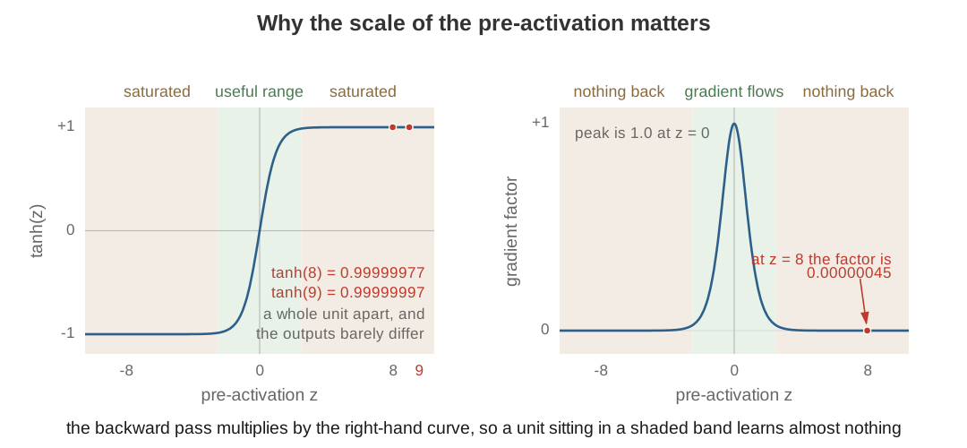
The right-hand panel is the one that matters for training. Backpropagation multiplies the incoming gradient by $1 - \tanh^2(z)$ as it passes back through the unit, and that factor is $1$ at $z = 0$ but only $0.00000045$ at $z = 8$. A unit sitting out in either shaded band is not broken, and its output is perfectly reasonable, but almost nothing gets past it on the way backwards, so the weights feeding it barely move.
You can address this by initializing the weights carefully so that the pre-activations start out at a reasonable scale. That works at the beginning of training. The difficulty is that the weights change as training proceeds, and the distribution of the pre-activations drifts with them. Careful initialization is a good starting point, not a lasting guarantee.
Batch normalization takes a more direct approach. Rather than arranging for the pre-activations to be well scaled and hoping they stay that way, it normalizes them explicitly at every forward pass: subtract the mean, divide by the standard deviation. The values entering the nonlinearity then have mean $0$ and variance $1$ by construction, at every step of training, no matter what the weights below have been doing.
Forcing every layer’s output to be exactly mean $0$ and variance $1$ would be too rigid, though. A unit that would benefit from being saturated some of the time has no way to get there. So the layer adds two learned parameters, a scale $\gamma$ and a shift $\beta$, which let the network move and stretch the distribution to wherever it is most useful. Normalization sets a sane default; $\gamma$ and $\beta$ let the network depart from it deliberately.
There is a cost, and it is the reason this post exists. The mean and the variance are computed over the batch, so the output for one example now depends on the other examples that happened to be in the batch with it. The examples are no longer processed independently. That coupling is what makes the backward pass interesting.
The forward pass
Let the batch contain $m$ examples, and write $x_1, x_2, \ldots, x_m$ for the values arriving at the layer. Batch normalization computes four things in order.
First, the mean of the batch:
\[\mu = \frac{1}{m} \sum_{i=1}^{m} x_i\]Second, the variance about that mean:
\[\sigma^2 = \frac{1}{m-1} \sum_{i=1}^{m} (x_i - \mu)^2\]The divisor is $m-1$ rather than $m$. That is Bessel’s correction, which makes this an unbiased estimate of the variance of the distribution the batch was drawn from. Some implementations divide by $m$ instead. The choice changes one constant in the gradient later, and we will note it when we get there.
Third, normalize each value:
\[\hat{x}_i = \frac{x_i - \mu}{\sqrt{\sigma^2 + \varepsilon}}\]Subtracting $\mu$ centres the batch at zero, and dividing by the standard deviation scales it to unit variance. The $\varepsilon$ is a small constant, typically $10^{-5}$, which keeps the denominator away from zero if the batch happens to have almost no variation.
Fourth, scale and shift:
\[y_i = \gamma \hat{x}_i + \beta\]$\gamma$ and $\beta$ are learned parameters, one pair per feature, shared across the batch. If the network wants the original distribution back it can learn $\gamma = \sqrt{\sigma^2 + \varepsilon}$ and $\beta = \mu$, so normalizing costs the layer no representational power.
In the notebook these are:
bnmeani  = 1/n*hprebn.sum(0, keepdim=True)      # mu
bndiff   = hprebn - bnmeani                     # x_i - mu
bndiff2  = bndiff**2
bnvar    = 1/(n-1)*(bndiff2).sum(0, keepdim=True)   # sigma^2
bnvar_inv= (bnvar + 1e-5)**-0.5                 # 1/sqrt(sigma^2 + eps)
bnraw    = bndiff * bnvar_inv                   # xhat_i
hpreact  = bngain * bnraw + bnbias              # y_i
So hprebn is $x$, hpreact is $y$, bngain is $\gamma$ and bnbias is $\beta$. We will use
the mathematical names from here on.
The computational graph
Here is the whole forward pass as a graph, with a batch of four. Four is small enough to draw every edge and large enough to show the pattern.
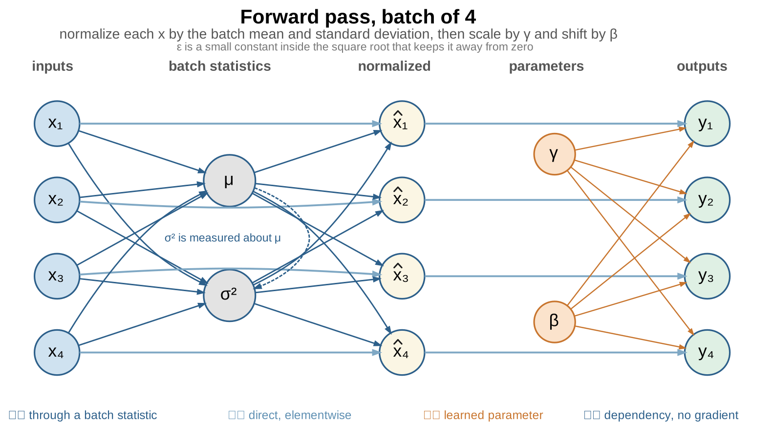
The shape of this graph is the whole story. Reading it left to right:
- Each $x_i$ has an edge into $\mu$ and an edge into $\sigma^2$. Every input contributes to both statistics, so those two nodes have a fan-in of $m$.
- $\mu$ and $\sigma^2$ each have an edge out to every $\hat{x}_j$. Both statistics are used by every normalized value, so those nodes have a fan-out of $m$.
- Each $x_i$ also has a direct edge to its own $\hat{x}_i$, the one in the numerator of $x_i - \mu$.
- There is a dashed edge from $\mu$ into $\sigma^2$, because the variance is measured about the mean. We will come back to it; it turns out to contribute nothing.
The consequence of the fan-in and fan-out together is that $x_2$ is connected to $\hat{x}_1$, $\hat{x}_3$ and $\hat{x}_4$, not only to $\hat{x}_2$. Changing one input shifts $\mu$ and $\sigma^2$, and those two numbers appear in every other example’s normalization.
The three routes out of one input
Pulling out just the edges that leave $x_2$ makes the point concrete:
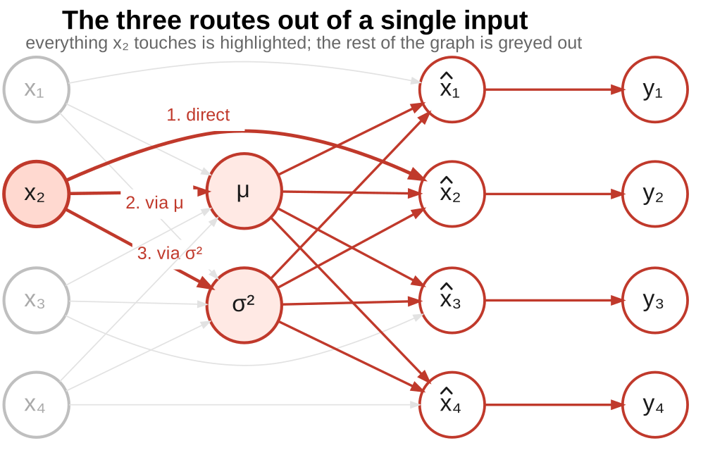
There are three ways for a change in $x_2$ to reach the loss:
- Directly, into its own $\hat{x}_2$.
- Through $\mu$, which then shifts all four normalized values.
- Through $\sigma^2$, which then rescales all four normalized values.
The rule from part 1 applies here without modification: a value used in several places collects a gradient from each of them, and the total is the sum. Three routes means three terms.
The three edges arriving at one normalized value
Looking in the other direction is just as useful:
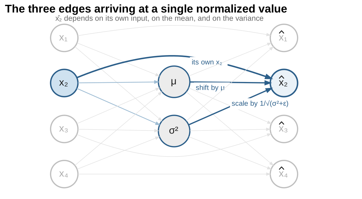
$\hat{x}_2$ depends on three things: its own $x_2$, the mean it is shifted by, and the variance it is scaled by. This is the picture behind the chain rule we will apply in a moment, because it tells us exactly which partial derivatives we need.
The gradients
We assume $\partial L / \partial y_i$ is already known, since it has been handed to us by whatever comes after this layer, and we want $\partial L / \partial x_i$. We will get there in four steps, following the graph backwards.
Step 1: the gradient at $\hat{x}_i$
The last operation was $y_i = \gamma \hat{x}_i + \beta$. That is an ordinary elementwise multiply, so:
\[\frac{\partial L}{\partial \hat{x}_i} = \frac{\partial L}{\partial y_i} \cdot \gamma\]Each $\hat{x}_i$ affects only its own $y_i$, so there is no sum here. This is the one step in the whole derivation where nothing interesting happens, and it is a good place to start because everything downstream is written in terms of this quantity. To keep the later formulas readable, give it a short name:
\[g_i \;=\; \frac{\partial L}{\partial \hat{x}_i} \;=\; \gamma \frac{\partial L}{\partial y_i}\]Step 2: the gradient at $\sigma^2$
Now the fan-out starts to matter. The variance is used by every normalized value, so the gradient arriving at $\sigma^2$ is a sum over the whole batch:
\[\frac{\partial L}{\partial \sigma^2} = \sum_{i=1}^{m} \frac{\partial L}{\partial \hat{x}_i} \cdot \frac{\partial \hat{x}_i}{\partial \sigma^2}\]For the local derivative, $\hat{x}_i = (x_i - \mu)(\sigma^2 + \varepsilon)^{-1/2}$, and treating $(x_i - \mu)$ as a constant with respect to $\sigma^2$:
\[\frac{\partial \hat{x}_i}{\partial \sigma^2} = (x_i - \mu) \cdot \left(-\tfrac{1}{2}\right)(\sigma^2 + \varepsilon)^{-3/2}\]The $-\tfrac{1}{2}$ and the $-3/2$ exponent both come from differentiating the power $(\sigma^2 + \varepsilon)^{-1/2}$. Putting it together:
\[\frac{\partial L}{\partial \sigma^2} = -\frac{1}{2} (\sigma^2 + \varepsilon)^{-3/2} \sum_{i=1}^{m} g_i \, (x_i - \mu)\]The sum says that every example gets a vote on how the variance should change, weighted by how far that example sits from the mean.
Step 3: the gradient at $\mu$
The mean is reached two ways: directly, through each $\hat{x}_i$, and indirectly, through $\sigma^2$, which is measured about $\mu$. That is the dashed edge in the graph. Both have to be counted:
\[\frac{\partial L}{\partial \mu} = \sum_{i=1}^{m} \frac{\partial L}{\partial \hat{x}_i} \frac{\partial \hat{x}_i}{\partial \mu} + \frac{\partial L}{\partial \sigma^2} \frac{\partial \sigma^2}{\partial \mu}\]The first local derivative is straightforward. Since $\hat{x}_i = (x_i - \mu)(\sigma^2 + \varepsilon)^{-1/2}$ and $\mu$ appears once with a minus sign:
\[\frac{\partial \hat{x}_i}{\partial \mu} = -(\sigma^2 + \varepsilon)^{-1/2}\]The second one is where something pleasant happens:
\[\frac{\partial \sigma^2}{\partial \mu} = \frac{\partial}{\partial \mu} \left[ \frac{1}{m-1} \sum_{i=1}^{m} (x_i - \mu)^2 \right] = \frac{-2}{m-1} \sum_{i=1}^{m} (x_i - \mu)\]And that sum is zero. Not approximately zero, exactly zero, because $\mu$ is by definition the value that makes the deviations cancel:
\[\sum_{i=1}^{m} (x_i - \mu) = \sum_{i=1}^{m} x_i - m\mu = m\mu - m\mu = 0\]So the whole second term vanishes, and the gradient at the mean is:
\[\frac{\partial L}{\partial \mu} = -(\sigma^2 + \varepsilon)^{-1/2} \sum_{i=1}^{m} g_i\]This is worth pausing on, because the graph and the algebra appear to disagree. The graph clearly shows an edge from $\mu$ to $\sigma^2$, and that edge is real: change $\mu$ and $\sigma^2$ does change. But $\mu$ is not a free variable. It is already sitting at the value that minimizes the sum of squared deviations, and at that point the derivative of $\sigma^2$ with respect to it is zero. The edge exists and carries nothing.
Step 4: the gradient at $x_i$
Now we can collect the three routes. Written out:
\[\frac{\partial L}{\partial x_i} = \underbrace{\frac{\partial L}{\partial \hat{x}_i} \frac{\partial \hat{x}_i}{\partial x_i}}_{\text{direct}} + \underbrace{\frac{\partial L}{\partial \mu} \frac{\partial \mu}{\partial x_i}}_{\text{via } \mu} + \underbrace{\frac{\partial L}{\partial \sigma^2} \frac{\partial \sigma^2}{\partial x_i}}_{\text{via } \sigma^2}\]Here is the backward graph, which is the forward graph with every edge reversed:
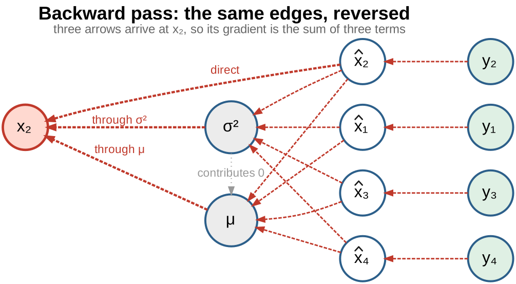
The three local derivatives are each a short calculation:
\[\frac{\partial \hat{x}_i}{\partial x_i} = (\sigma^2 + \varepsilon)^{-1/2} \qquad \frac{\partial \mu}{\partial x_i} = \frac{1}{m} \qquad \frac{\partial \sigma^2}{\partial x_i} = \frac{2(x_i - \mu)}{m-1}\]The first is the scaling factor. The second says each example contributes $1/m$ of the mean. The third comes from differentiating one term of the variance sum.
Substituting everything in gives a long expression:
\[\frac{\partial L}{\partial x_i} = g_i (\sigma^2 + \varepsilon)^{-\frac{1}{2}} \;-\; \frac{(\sigma^2 + \varepsilon)^{-\frac{1}{2}}}{m} \sum_{j=1}^{m} g_j \;-\; \frac{(\sigma^2+\varepsilon)^{-\frac{3}{2}}}{m-1} (x_i - \mu) \sum_{j=1}^{m} g_j (x_j - \mu)\]It looks unwieldy, but it simplifies. Notice that $(x_i - \mu)(\sigma^2 + \varepsilon)^{-1/2}$ is just $\hat{x}_i$, and the same substitution applies inside the sum. Factoring out $(\sigma^2 + \varepsilon)^{-1/2}$ and rewriting:
\[\frac{\partial L}{\partial x_i} = \frac{1}{\sqrt{\sigma^2 + \varepsilon}} \left[ g_i \;-\; \frac{1}{m}\sum_{j=1}^{m} g_j \;-\; \frac{m}{m-1}\,\hat{x}_i \cdot \frac{1}{m}\sum_{j=1}^{m} g_j \hat{x}_j \right]\]Reading the result
That final form is short enough to read as three instructions, and each one matches a route in the graph:
\[\frac{\partial L}{\partial x_i} = \frac{1}{\sqrt{\sigma^2 + \varepsilon}} \Big[ \underbrace{g_i}_{\text{direct}} \;-\; \underbrace{\operatorname{mean}(g)}_{\text{via } \mu} \;-\; \underbrace{\tfrac{m}{m-1}\,\hat{x}_i \operatorname{mean}(g \hat{x})}_{\text{via } \sigma^2} \Big]\]Take the incoming gradient, subtract its mean, then subtract its component along $\hat{x}$, and rescale. The two subtractions are not arbitrary corrections; they are exactly the $\mu$ path and the $\sigma^2$ path.
The middle term is the more intuitive of the two. If every $g_j$ pointed the same way, the layer would be trying to shift the whole batch up or down together. Normalization removes the mean, so that shift has no effect on the output, and the gradient reflects that by removing the mean of $g$ before passing it back.
The last term does the same thing for scale. If $g$ is proportional to $\hat{x}$, the layer is trying to stretch the batch. Normalization fixes the variance, so stretching has no effect either, and the corresponding component is removed. The factor $\frac{m}{m-1}$ is the Bessel correction following through; with the biased variance ($\frac{1}{m}$ instead of $\frac{1}{m-1}$) it becomes $1$ and the expression is perfectly symmetric.
Written in terms of $\partial L / \partial y_i$ instead of $g_i$, this is the form in the video:
\[\frac{\partial L}{\partial x_i} = \frac{\gamma (\sigma^2 + \varepsilon)^{-\frac{1}{2}}}{m} \left[ m \frac{\partial L}{\partial y_i} - \sum_{j=1}^{m} \frac{\partial L}{\partial y_j} - \frac{m}{m-1} \hat{x}_i \sum_{j=1}^{m} \frac{\partial L}{\partial y_j} \hat{x}_j \right]\]The two are the same expression; the first is factored to make the three terms readable, the second to make the code obvious.
The gradients for $\gamma$ and $\beta$
These are easier, because $\gamma$ and $\beta$ are shared across the batch and used once per example. Each collects a sum over the batch:
\[\frac{\partial L}{\partial \gamma} = \sum_{i=1}^{m} \frac{\partial L}{\partial y_i} \hat{x}_i \qquad \frac{\partial L}{\partial \beta} = \sum_{i=1}^{m} \frac{\partial L}{\partial y_i}\]In code
dxhat = bngain * dhpreact                      # g_i

dhprebn = bnvar_inv/n * (
      n*dxhat                                  # direct
    - dxhat.sum(0)                             # via the mean
    - n/(n-1) * bnraw * (dxhat*bnraw).sum(0)   # via the variance
)

dbngain = (dhpreact * bnraw).sum(0, keepdim=True)
dbnbias = dhpreact.sum(0, keepdim=True)
And the fused form, with $\gamma$ folded in, is the one line from the notebook:
dhprebn = bngain*bnvar_inv/n * (n*dhpreact - dhpreact.sum(0)
                               - n/(n-1)*bnraw*(dhpreact*bnraw).sum(0))
Comparing against autograd gives a maximum absolute difference of about $10^{-9}$, which is floating point noise rather than a mistake in the derivation.
Wrapping up
Batch normalization looks more complicated than the operations in the earlier posts, and in one specific way it is: the batch statistics turn a set of independent examples into a set of coupled ones. But the rule for handling that is the same rule as always. Count the routes from the value to the loss, differentiate along each one, and add.
The graph tells you how many terms to expect before you do any calculus. Three edges leave $x_i$, so there are three terms. The fan-out from $\mu$ and $\sigma^2$ tells you two of those terms will contain sums over the batch. And the one edge that looks like a fourth route, from $\mu$ into $\sigma^2$, turns out to carry zero, because $\mu$ already sits where the deviations cancel.
What comes out the other end is short enough to read: remove the mean of the gradient, remove its component along $\hat{x}$, and rescale. The layer refuses to pass back any gradient that would merely shift or stretch the batch, which is precisely what you would expect from a layer whose job is to fix the shift and the stretch.