Context: Like the earlier posts in this series, this one comes out of Andrej Karpathy’s Becoming a Backprop Ninja (Part 4 of the spelled-out intro series), where you hand-write every backward pass instead of calling
.backward(). These notes are the slower explanation I want on hand the next time I go back to the video. If you have not watched it, start there:

Part 1 looked at a broadcast in the forward pass and found a sum waiting in the backward pass. This post runs the same setup in the other direction.
B = A.sum(dim=1, keepdim=True) # A is (2, 2), B is (2, 1)
A 2x2 goes in, a 2x1 comes out. Each row of A gets collapsed into a single number. Four values in, two values out.
The gradient has to travel the opposite way, from a 2x1 back into a 2x2. Two numbers have to become four. The only thing that can do that is a copy, and copying a column across is exactly what broadcasting is.
This is the pairing that makes both halves easy to remember: a sum in the forward pass is a broadcast in the backward pass, and a broadcast in the forward pass is a sum in the backward pass. The two operations are duals of each other. If you can derive one, you already have the other.
Writing the forward pass out longhand
Name every element rather than using numbers. A is 2x2:
A = | A11  A12 |
    | A21  A22 |
Summing along dim=1 adds up each row:
B1 = A11 + A12
B2 = A21 + A22
so B is a 2x1 column:
B = | B1 |
    | B2 |
The keepdim=True is what keeps it a (2, 1) column rather than a flat (2,) vector. That distinction matters later on and I will come back to it.
Here is the same thing as a picture, both rows drawn out:
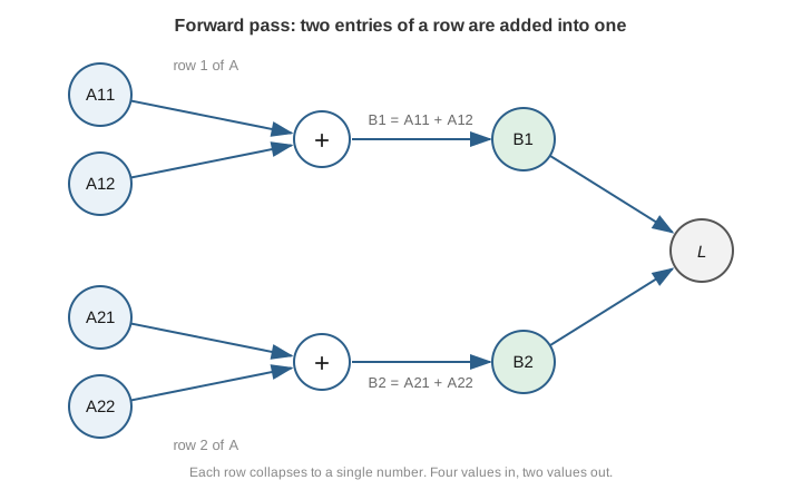
Two things to notice. Each A element has exactly one arrow leaving it, so nothing is being reused here. And the plus nodes have two arrows coming in and one going out, which is where the collapsing happens.
What we are given, and what we want
Assume B feeds the rest of the network and eventually a scalar loss L. Backprop hands us:
G = dL/dB
which is the same shape as B, so 2x1, with entries G1 and G2.
We need dL/dA, which must be 2x2 because A is 2x2.
Two numbers have to turn into four. Hold that thought, it will answer the question on its own in a minute.
The derivation
Take A11. Where does it appear in the output? In exactly one place, B1 = A11 + A12. So the chain rule has a single path to walk:
dL/dA11 = dL/dB1 * dB1/dA11
The local derivative dB1/dA11 is 1. Addition does not scale anything: bump A11 by epsilon and B1 goes up by exactly epsilon, no more and no less. Having A12 sitting next to it in the sum changes nothing about how B1 responds to a wiggle in A11.
dL/dA11 = G1 * 1 = G1
Now do A12. It also appears in exactly one place, also B1, and also with a local derivative of 1:
dL/dA12 = G1 * 1 = G1
The same value. Not a coincidence, and not an accident of this example. A11 and A12 both feed the same output through the same kind of edge, so the same gradient comes back to both of them.
Row 2 works identically:
dL/dA21 = G2 dL/dA22 = G2
Putting it together:
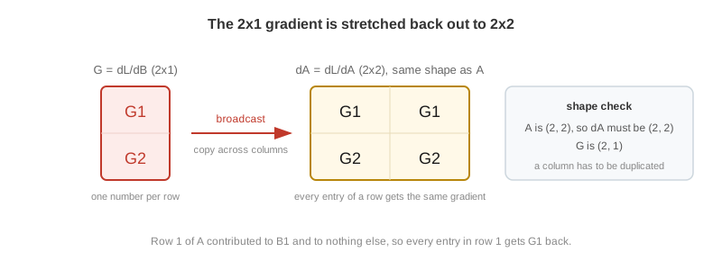
dA = | G1  G1 |
     | G2  G2 |
which is G, copied across the columns.
The backward graph
Reverse every arrow in the forward diagram and the picture explains itself:
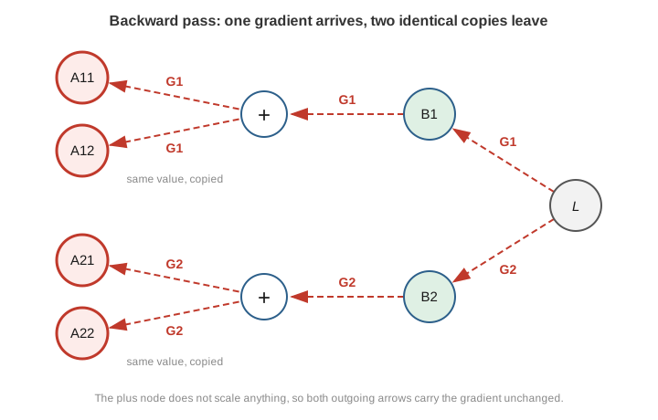
One arrow arrives at the plus node carrying G1. Two arrows leave it, and both carry G1. The plus node has no multiplier attached to it, so there is nothing to scale the gradient by on the way out.
That fan-out on the backward side is the mirror of what happened in part 1. There, B1 fanned out in the forward pass and the gradients came back and added together at the node. Here, the plus node fans out in the backward pass and the gradient gets copied. Same picture, read from the other end.
In matrix form:
Any of these will do it in code:
dA = G * np.ones((1, 2))     # explicit multiply by ones
dA = np.broadcast_to(G, A.shape)
dA = G + np.zeros_like(A)    # add zero, let broadcasting expand
In PyTorch, G.expand(-1, 2) does the same without allocating anything, which is what autograd actually does internally.
The duality
Lining the two posts up next to each other:
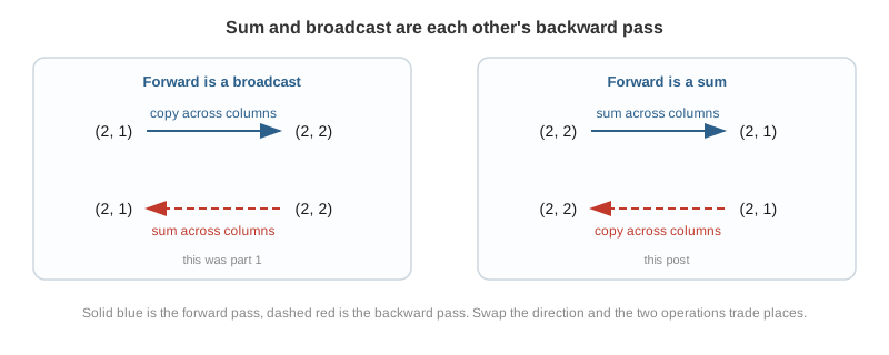
This is a real duality and it is worth naming, because it turns two things to memorize into one:
- Sum forward, broadcast backward. Several values feed one output through addition, so that one gradient is handed to every input untouched.
- Broadcast forward, sum backward. One value feeds several outputs, so the gradients from all of those places add up when they come home.
Both statements are the same fact about the chain rule, viewed from opposite ends. A copy node run in reverse is an add node, and an add node run in reverse is a copy node.
There is a slightly deeper reason for this, if you want it. Both operations are linear, and the backward pass of a linear map is its transpose. Broadcasting a (2, 1) into a (2, 2) and summing a (2, 2) back into a (2, 1) are described by the same matrix of ones, just transposed. That is why they keep showing up as a pair.
Shape checking
The shape check from the earlier posts settles this one before you write down a single derivative.
A gradient always has the same shape as the thing it is the gradient of:
A is (2, 2)   ->   dA must be (2, 2)
G is (2, 1)
A (2, 1) has to become a (2, 2). There is no way to invent new information, so the only candidate is duplicating what is already there, which is broadcasting.
Compare that to part 1, where dB had to be (3, 1) while G was (3, 3), and columns had to disappear, so a sum was the only option. Whenever a broadcast dimension has to grow, you copy. Whenever it has to shrink, you sum. The shapes pick the operation for you.
A note on keepdim
This is the one place the operation bites in practice:
B = A.sum(dim=1)                  # shape (2,)
B = A.sum(dim=1, keepdim=True)    # shape (2, 1)
Without keepdim, the dimension is gone rather than flattened to size 1, and a (2,) tensor broadcasts along the last axis, not the first. So A / A.sum(dim=1) silently divides each column by the wrong thing instead of raising an error. It is a bug that runs perfectly happily and gives you nonsense.
Keep the dimension. It makes the broadcast go the direction you intended, and it keeps the gradient shapes lining up without any fiddling.
Where you actually hit this
The denominator of a softmax:
counts_sum = counts.sum(dim=1, keepdim=True)     # sum forward
probs = counts / counts_sum                      # broadcast forward
Both halves of the duality inside two lines. The first line sums across a row, so its backward pass broadcasts. The second line broadcasts a column across, so its backward pass sums. When you hand-write the backward pass for a softmax and one of the terms has an unexpected .sum() or an unexpected copy in it, this is usually why.
The same pair shows up in layer norm, in attention, and anywhere else a per-row statistic is computed and then applied back to the row.
Verifying it
import torch

A = torch.randn(2, 2, requires_grad=True)

B = A.sum(dim=1, keepdim=True)     # B is (2, 1)
G = torch.randn(2, 1)              # pretend upstream gradient
B.backward(G)

print(torch.allclose(A.grad, G.expand(-1, 2)))     # True
print(A.grad)
Which prints something like:
True
tensor([[-1.0845, -1.0845],
        [-1.3986, -1.3986]])
Each row holds the same number twice, which is the copy showing up in the output.
Wrapping up
Four posts in, and every one of them has come down to the same question: where does this variable appear in the forward pass, and how many times?
- Used once, and just added: the gradient arrives unchanged. That is every element of
Ahere. - Used many times: the gradients add. That was the broadcast vector in part 1 and the bias in part 3.
- Used conditionally: the gradient only flows down the path that was actually taken, which was the max in part 2.
Sum and broadcast are the cleanest example of the pattern because they are each other’s mirror image.