I wanted a small answer to a concrete question: if I change the activation inside the feed-forward network of a GPT-2-sized model, what happens to its loss curve? I used Karpathy’s build-nanoGPT as the starting point, kept the model and training recipe controlled, and ran GELU, SwiGLU, and ReLU versions on one RTX 4090.
The result is not a general ranking of activations. It is one seed, one model size, one data slice, and thirty minutes of active training for each variant. It does show a useful tradeoff: in this run, parameter-matched SwiGLU processed fewer tokens than GELU but reached lower held-out loss.
Where GELU sits in build-nanoGPT
A Transformer block has an attention sublayer and a feed-forward network, often abbreviated MLP for multi-layer perceptron. Attention lets a token mix information from earlier tokens. The MLP then transforms that token’s resulting vector independently of the other positions.
In the baseline model, the MLP first expands an input vector $x$, applies the Gaussian Error Linear Unit, or GELU, then projects the result back down:
\[\operatorname{MLP}_{\text{GELU}}(x) = W_{\text{down}}\operatorname{GELU}(W_{\text{up}}x+b_{\text{up}})+b_{\text{down}}.\]The local build-nanoGPT source implements that path with nn.GELU(approximate='tanh'). The figure shows the standard definition, $\operatorname{GELU}(x)=x\Phi(x)$, where $\Phi(x)$ is the cumulative probability of a standard normal variable being at most $x$. PyTorch uses the tanh approximation because it is inexpensive to evaluate while closely tracking that curve.
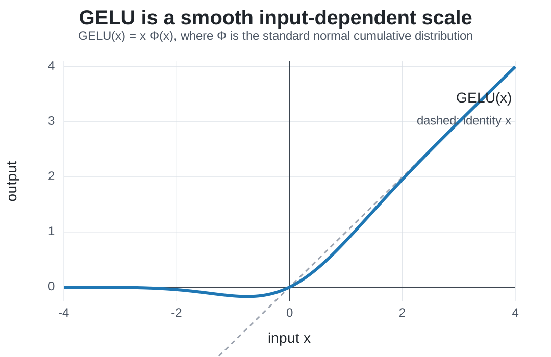
Figure 1. GELU smoothly scales each scalar activation. The code uses PyTorch’s tanh approximation of this standard curve.
For a strongly positive input, GELU is close to the identity function: it lets that component through. For a negative input, it reduces the component smoothly rather than applying ReLU’s hard cutoff at zero. That smooth scaling is all the ordinary GELU MLP has between its two learned linear projections.
SwiGLU adds a learned gate
SwiGLU is a gated linear unit variant. It creates two expanded vectors from the same input. One is a candidate value, and the other becomes a gate after the Sigmoid Linear Unit, or SiLU, function:
\[u = W_{\text{up}}x+b_{\text{up}}, \qquad g = W_{\text{gate}}x+b_{\text{gate}},\] \[\operatorname{SiLU}(g)=g\,\sigma(g), \qquad \operatorname{MLP}_{\text{SwiGLU}}(x)=W_{\text{down}}(\operatorname{SiLU}(g)\odot u)+b_{\text{down}}.\]Here $\sigma$ is the sigmoid function and $\odot$ means element-wise multiplication. If these vectors have 2,048 components, component 731 of SiLU(g) multiplies component 731 of u; it does not combine every component with every other component. The output projection then mixes the resulting 2,048 scaled components back into the model’s 768-component embedding space.
The word gate is useful, but it should not suggest a binary on/off switch. Suppose one small slice has $u=[0.5, 3.0, -1.0]$ and $g=[2.0, -2.0, 0.0]$. Then $\operatorname{SiLU}(g)\approx[1.76,-0.24,0.0]$, and the element-wise product is approximately $[0.88,-0.71,0.0]$. The first candidate component is amplified, the second changes sign and is reduced, and the third is removed. The learned output projection decides how to use those resulting values. This is only a three-number illustration, not a claim about what any particular trained component represents.
Think of the representation for the phrase “river bank” as carrying several possible interpretations. The candidate vector $u$ can contain directions useful for terrain, water, money, grammar, and many other learned features. The gate supplies a second input-dependent value for each direction. In this toy picture, features supporting the river sense can keep flowing while features that would support the financial sense can be reduced. The model does not contain a literal river_feature or money_feature; the example describes how a learned gate can select among context-dependent directions.
GELU also changes each component according to its input. SwiGLU differs because it learns a separate projection to decide that scaling. That extra projection gives the MLP a richer conditional transformation. To keep the comparison parameter-matched, the SwiGLU projections are narrower; SiLU and the element-wise gate still add operations to the MLP.
Making sure the number of parameters is apples to apples
Adding the gate without changing anything else would give SwiGLU substantially more parameters than GELU. I instead reduced the SwiGLU hidden width. The GPT-2-small embedding width is 768. GELU uses a 3,072-wide MLP with two weight matrices, so its MLP matrix count per block is:
\[2\times768\times3072.\]SwiGLU uses three matrices, up, gate, and down. Choosing width 2,048 gives:
The matrix counts are exactly equal. Keeping biases leaves SwiGLU with 124,488,192 trainable parameters, versus 124,475,904 for GELU, a difference of 12,288 parameters or 0.00987%. ReLU keeps GELU’s 3,072-wide two-matrix MLP and has exactly the same parameter count as GELU.
The experiment copied GELU’s non-MLP initial tensors into the SwiGLU model. That matters because changing the MLP shape would otherwise shift initialization of later block tensors, including attention tensors in subsequent blocks. The runner copies every non-MLP tensor, including the embeddings, so the shared components start identically. ReLU has the same tensor shapes as GELU, so its initial weights match GELU exactly.
The training run
Each variant used the GPT-2-small shape: 12 Transformer blocks, 12 attention heads, and an embedding width of 768. The model keeps 1,024 learned position embeddings, while this short single-GPU comparison feeds sequences of $T=256$ tokens. The smaller sequence length is part of the experiment recipe, not a limit of build-nanoGPT. Each optimizer update processes two micro-batches of 16 sequences. A micro-batch is a smaller piece of an optimizer batch: the runner processes two 16-sequence micro-batches separately, averages their gradients, then applies one weight update, reducing peak memory for the effective 32-sequence batch:
\[2\times16\times256=8{,}192\]next-token predictions per update. All three runs used the same deterministic token order, seed 1337, BF16 autocast with FP32 weights, fused AdamW, the same warmup and constant learning rate, and eager PyTorch without torch.compile.
I trained each model for 1,800 seconds of synchronized active update time. Every roughly sixty seconds, the runner evaluated the same fixed 65,536-token training prefix and the same fixed 65,536-token held-out validation prefix. With a 16-by-256 micro-batch, each evaluation contains 16 equal batches of 4,096 token predictions. Cross-entropy is measured in nats per token, the natural-log unit of next-token surprise. Lower values mean the model assigns more probability to the observed next tokens.
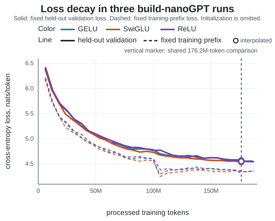
Figure 2. Recorded loss curves from the three runs. Color identifies the activation, solid lines are held-out validation, and dashed lines are the fixed training prefix. The vertical marker is the 176.2-million-token shared comparison; open circles are interpolated and the filled orange circle is SwiGLU’s measured value.
The SwiGLU variant completed fewer updates in the same thirty-minute window: 176,218,112 tokens, compared with 186,130,432 for GELU and 187,334,656 for ReLU. To account for this, we draw the X-axis as number of tokens trained, instead of time.
The sharp fall in each dashed fixed-training curve just after 100 million tokens coincides with the first wrap to the beginning of the 100-million-token training array. The evaluated training prefix is then seen again. The validation curve does not receive that direct second exposure.
| Activation | Fixed training loss | Held-out validation loss |
|---|---|---|
| GELU | 4.36397 | 4.57345 |
| SwiGLU | 4.35385 | 4.53739 |
| ReLU | 4.34065 | 4.55372 |
At the shared token budget, SwiGLU improved validation loss over GELU by 0.03606 nats per token. ReLU reached the lowest fixed-training loss while SwiGLU reached the lowest held-out loss. That distinction matters: fitting the fixed training prefix more closely is not the same thing as predicting the validation prefix better.
Conclusion
The displayed SwiGLU curve is smoother, and it reaches a slightly lower held-out validation loss than GELU at the shared 176.2-million-token point. The MLP computes a separate gate projection, applies SiLU to it, and multiplies it element by element with the value path. In this eager-PyTorch setup, the parameter-matched SwiGLU run trained more slowly.
References and source notes
- Dan Hendrycks and Kevin Gimpel, Gaussian Error Linear Units (GELUs).
- Noam Shazeer, GLU Variants Improve Transformer, which motivates the parameter-matched SwiGLU width.
- Andrej Karpathy, build-nanoGPT at the pinned baseline revision.